Probability Trees and Conditional Expectations

Probability trees and conditional expectations are essential tools in quantitative finance, particularly for the CFA Exam. Probability trees visually break down sequential events, allowing analysts to map and calculate complex probabilities in steps. Conditional expectations refine outcome predictions based on specific conditions, providing a deeper understanding of expected returns and risk. Together, these methods are valuable for assessing financial scenarios, predicting asset behaviors, and updating investment probabilities as new information arises. Mastery of these concepts supports informed, data-driven decision-making in finance.

Learning Objectives

In studying “Probability Trees and Conditional Expectations” for the CFA Exam, you should aim to understand how probability trees break down complex, sequential events into manageable steps, illustrating each outcome’s probability. Learn to calculate conditional probabilities, which help assess the likelihood of an event given prior information, essential for risk assessment. Analyze how expected values provide a weighted average of outcomes, guiding investment decisions. Additionally, explore how Bayes’ theorem updates probabilities with new information, refining predictions. Mastering these tools will enable you to interpret conditional outcomes, evaluate financial scenarios, and improve decision-making in real-world CFA applications.

Probability Trees

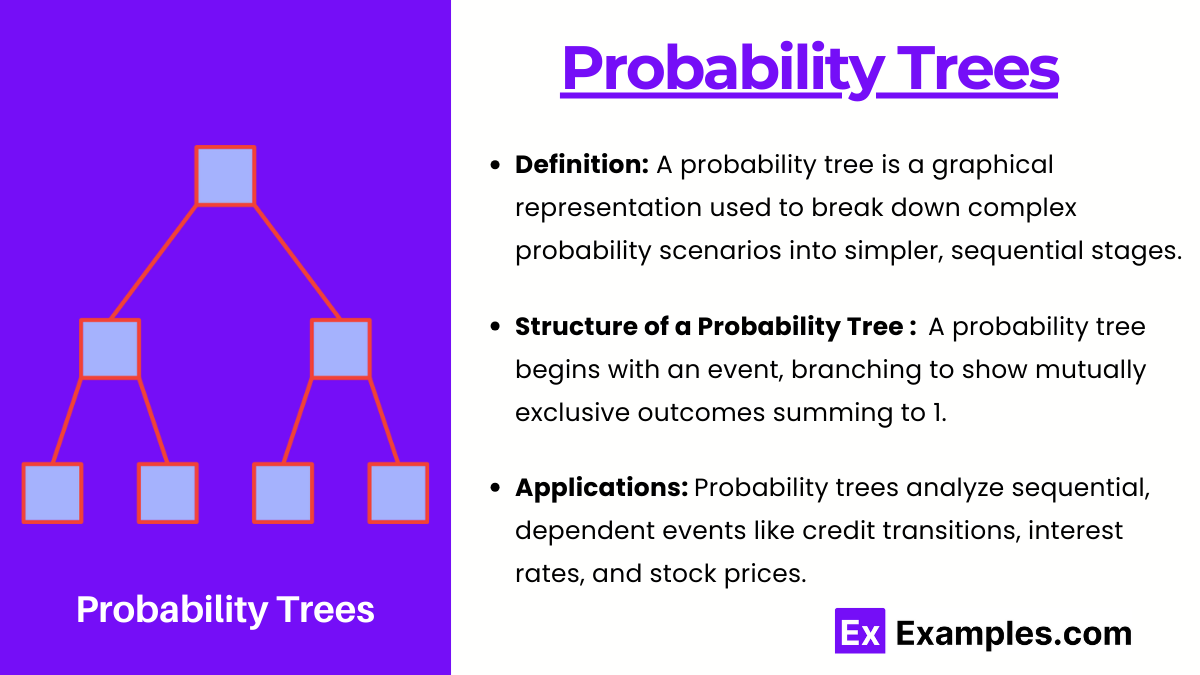
• Definition: A probability tree is a graphical representation used to break down complex probability scenarios into simpler, sequential stages. Each branch represents a possible outcome, and the probability of each event is noted along the branches, making it easier to calculate the likelihood of specific sequences of events.
• Structure of a Probability Tree: The tree starts with an initial event and branches out to show all possible outcomes, which may lead to further branches (subsequent events). Each level of branches is mutually exclusive, and all probabilities at a level should sum to 1.
• Applications: Probability trees are especially useful for analyzing events that are sequential and dependent on previous outcomes, such as understanding credit rating transitions, interest rate changes, and stock price movements in finance.

Conditional Probability

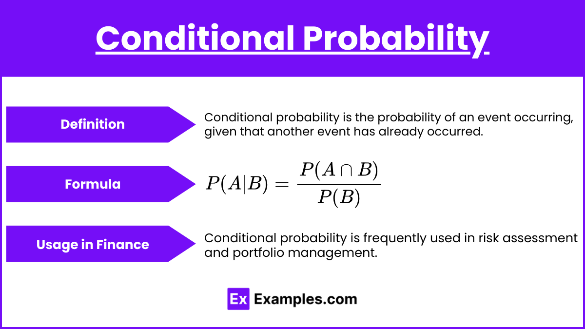
• Definition: Conditional probability is the probability of an event occurring, given that another event has already occurred. It’s expressed as P(A∣B), representing the probability of event A given that B has occurred.
• Formula: The formula for conditional probability is:
• where P(A∩B) is the joint probability of A and B happening together, and P(B) is the probability of B.
• Usage in Finance: Conditional probability is frequently used in risk assessment and portfolio management. For example, it helps determine the likelihood of a bond defaulting given a change in its credit rating, or the probability of a stock appreciating given recent market movements.

Expected Value (Expectation)

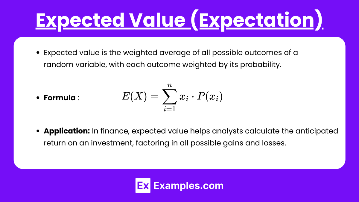
• Expected value is the weighted average of all possible outcomes of a random variable, with each outcome weighted by its probability. It is a key metric in assessing the long-term average outcome of an uncertain event.
• Formula: For a random variable X with outcomes x1​,x2​,…,xn​ and probabilities P(x1​),P(x2​),…,P(xn​), the expected value E(X) is:
• Application: In finance, expected value helps analysts calculate the anticipated return on an investment, factoring in all possible gains and losses. It is fundamental to investment decision-making and risk management.

Bayes’ Theorem and Updating Probabilities

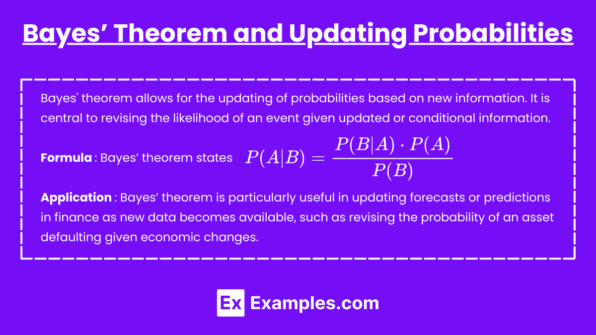
• Definition: Bayes’ theorem allows for the updating of probabilities based on new information. It is central to revising the likelihood of an event given updated or conditional information.
• Formula: Bayes’ theorem states:
• Application: Bayes’ theorem is particularly useful in updating forecasts or predictions in finance as new data becomes available, such as revising the probability of an asset defaulting given economic changes.

Examples

Example1. Credit Rating Transition Analysis Using Probability Trees

An analyst is studying a company’s credit rating, which can move from an “A” rating to either a “B” or “BB” rating next year, with probabilities of 0.3 and 0.7, respectively. Using a probability tree, the analyst maps out potential rating transitions over two years. This tree helps estimate the likelihood of specific rating sequences, which informs risk assessment and valuation of the company’s debt. By visualizing transitions over multiple periods, probability trees provide a structured approach to tracking credit rating changes and their potential impact on investment.

Example 2. Conditional Probability of Default in a Recession Scenario

An investor wants to know the probability of a bond defaulting if a recession occurs. Data shows that if there is a recession, the probability of default (event A) is 20%, but without a recession, the probability drops to 5%. Using conditional probability, the investor calculates P(default∣recession)=0.20, aiding in evaluating the bond’s risk in different economic scenarios. Conditional probabilities like this help investors refine risk estimates based on real-world events, such as economic downturns, improving their decision-making process.

Example 3. Expected Return on Investment in a Bull vs. Bear Market

A portfolio manager estimates the expected return of a stock based on market conditions. In a bull market, the stock is expected to return 15%, while in a bear market, it is likely to lose 5%. If the probability of a bull market is 70%, the expected return is calculated as:

E(Return) = (0.70×15%) + (0.30×−5%) = 9%

This conditional expectation gives the manager a better estimate of the stock’s likely performance under different market conditions, allowing for more informed portfolio allocation.

Example 4. Decision-Making with Bayes’ Theorem for Stock Price Prediction

An analyst wants to update the probability of a stock appreciating based on recent news. Initially, there is a 40% chance the stock will appreciate (prior probability). New information suggests a 70% probability of the stock appreciating if positive news is announced. Using Bayes’ Theorem, the analyst updates the probability of appreciation, enhancing forecast accuracy. Bayesian updating is especially valuable for incorporating new data into investment decisions, making probability predictions more relevant as market information changes.

Example 5. Portfolio Diversification Strategy Based on Asset Correlations

A financial advisor assesses a portfolio where two assets, A and B, have a historical correlation of -0.5, suggesting an inverse relationship. By calculating conditional expectations, the advisor determines that if Asset A experiences a negative return, Asset B has a high likelihood of delivering a positive return. Using this conditional insight, the advisor recommends including both assets to balance overall portfolio volatility. Conditional expectations allow investors to strategically pair assets, enhancing portfolio stability through diversification.

Practice Questions

Question 1

An investor is analyzing the potential outcomes of a stock’s performance over two years. The probability that the stock will increase in the first year is 60%, and if it increases in the first year, there is a 50% chance it will increase in the second year. What is the probability that the stock will increase in both years?

A) 10%
B) 30%
C) 50%
D) 60%

Answer: B) 30%

Explanation: To find the probability of the stock increasing in both years, we multiply the probability of an increase in the first year by the conditional probability of an increase in the second year given an increase in the first year.

P(Increase in both years) = P(Increase in Year 1) × P(Increase in Year 2 | Increase in Year 1) = 0.60 × 0.50 = 0.30or 30%

This approach is a basic application of conditional probability, where we account for the sequential nature of the events. The probability tree model helps visualize these types of sequential events.

Question 2

A financial analyst is studying a company with a 40% chance of a favorable earnings report. If the report is favorable, there is a 75% chance the company’s stock price will increase. What is the probability that the earnings report is favorable and the stock price increases?

A) 30%
B) 40%
C) 50%
D) 75%

Answer: A) 30%

Explanation: The probability of both events (a favorable report and a stock price increase) occurring is found by multiplying the probability of a favorable earnings report by the conditional probability of a stock price increase given a favorable report.

P(Favorable report and price increase) = P(Favorable report) × P(Price increase | Favorable report) = 0.40 × 0.75 = 0.30or 30%

Question 3

An investment manager evaluates two assets, A and B. Asset A has a 0.2 probability of yielding a negative return. If Asset A yields a negative return, there is a 0.6 probability that Asset B will yield a positive return. What is the probability that Asset A yields a negative return and Asset B yields a positive return?

A) 8%
B) 12%
C) 15%
D) 18%

Answer: B) 12%

Explanation: To determine the joint probability of Asset A yielding a negative return and Asset B yielding a positive return, we multiply the probability of Asset A having a negative return by the conditional probability that Asset B has a positive return given that Asset A has a negative return.

P(A negative and B positive) = P(A negative) × P(B positive | A negative) = 0.20 × 0.60 = 0.12or 12%

This calculation demonstrates the application of conditional expectations in evaluating portfolio diversification and the likelihood of different asset combinations delivering balanced returns. Such probability assessments are key in portfolio construction and risk management in the CFA curriculum.