AP® Calculus AB Cheat Sheet

This AP Calculus AB Cheat Sheet provides a concise overview of essential formulas, key concepts, and critical information from the AP Calculus AB curriculum. Covering all major topics, it simplifies complex ideas into easy-to-understand points, helping students quickly review and solidify their understanding. With important calculus formulas, theorems, and example problems, students can effectively apply these concepts to both multiple-choice and free-response questions. Organized into clear sections with step-by-step explanations, this cheat sheet is a valuable tool for mastering the exam and achieving top scores in AP Calculus AB.

Free AP Calculus AB Practice Test

Download AP Calculus AB Cheatsheet – Pdf

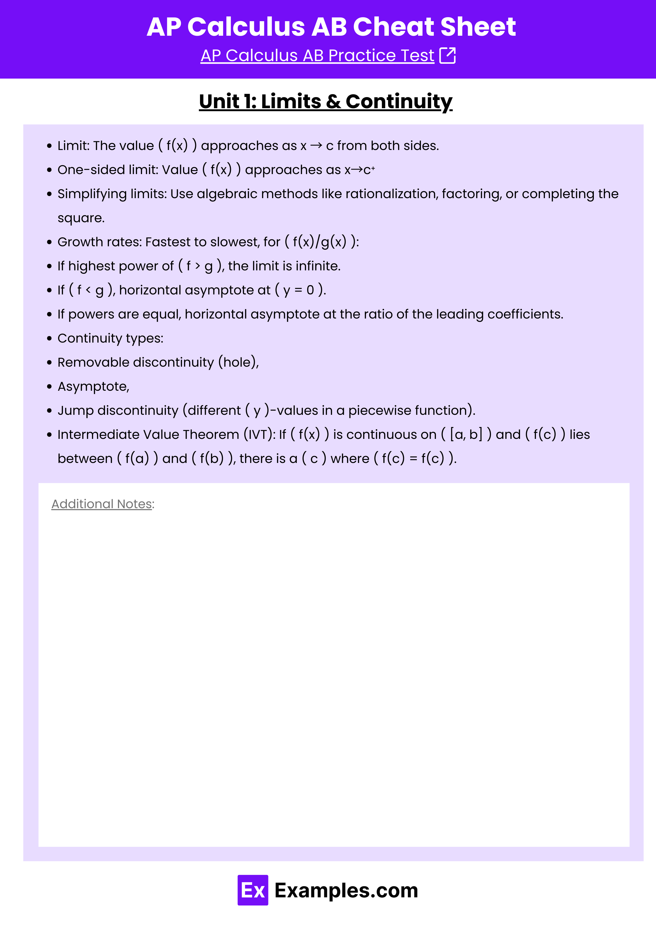
Unit 1: Limits & Continuity

• Limit: The value ( f(x) ) approaches as x → c from both sides.
• One-sided limit: Value ( f(x) ) approaches as x→c⁺
• Simplifying limits: Use algebraic methods like rationalization, factoring, or completing the square.
• Growth rates: Fastest to slowest, for ( f(x)/g(x) ):
• If highest power of ( f > g ), the limit is infinite.
• If ( f < g ), horizontal asymptote at ( y = 0 ).
• If powers are equal, horizontal asymptote at the ratio of the leading coefficients.
• Continuity types:
• Removable discontinuity (hole),
• Asymptote,
• Jump discontinuity (different ( y )-values in a piecewise function).
• Intermediate Value Theorem (IVT): If ( f(x) ) is continuous on ( [a, b] ) and ( f(c) ) lies between ( f(a) ) and ( f(b) ), there is a ( c ) where ( f(c) = f(c) ).

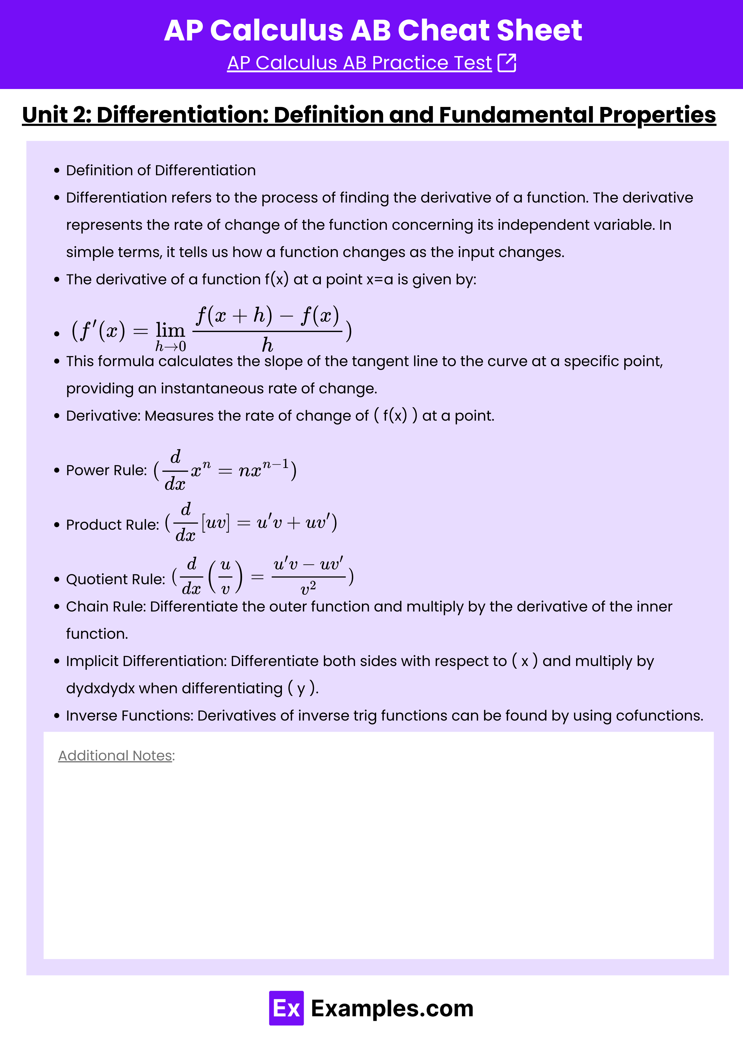
Unit 2: Differentiation: Definition and Fundamental Properties

Definition of Differentiation

Differentiation refers to the process of finding the derivative of a function. The derivative represents the rate of change of the function concerning its independent variable. In simple terms, it tells us how a function changes as the input changes.

The derivative of a function f(x) at a point x=a is given by:

\( f'(x) = \lim_{h \to 0} \frac{f(x + h) – f(x)}{h} \)

This formula calculates the slope of the tangent line to the curve at a specific point, providing an instantaneous rate of change.

• Derivative: Measures the rate of change of ( f(x) ) at a point.
• Power Rule: \(\frac{d}{dx} x^n = n x^{n-1}\)
• Product Rule: \(\frac{d}{dx} [uv] = u’v + uv’ \)
• Quotient Rule: \(\frac{d}{dx} \left( \frac{u}{v} \right) = \frac{u’v – uv’}{v^2}\)
• Chain Rule: Differentiate the outer function and multiply by the derivative of the inner function.
• Implicit Differentiation: Differentiate both sides with respect to ( x ) and multiply by \(\frac{dy}{dx}\) when differentiating ( y ).
• Inverse Functions: Derivatives of inverse trig functions can be found by using cofunctions.

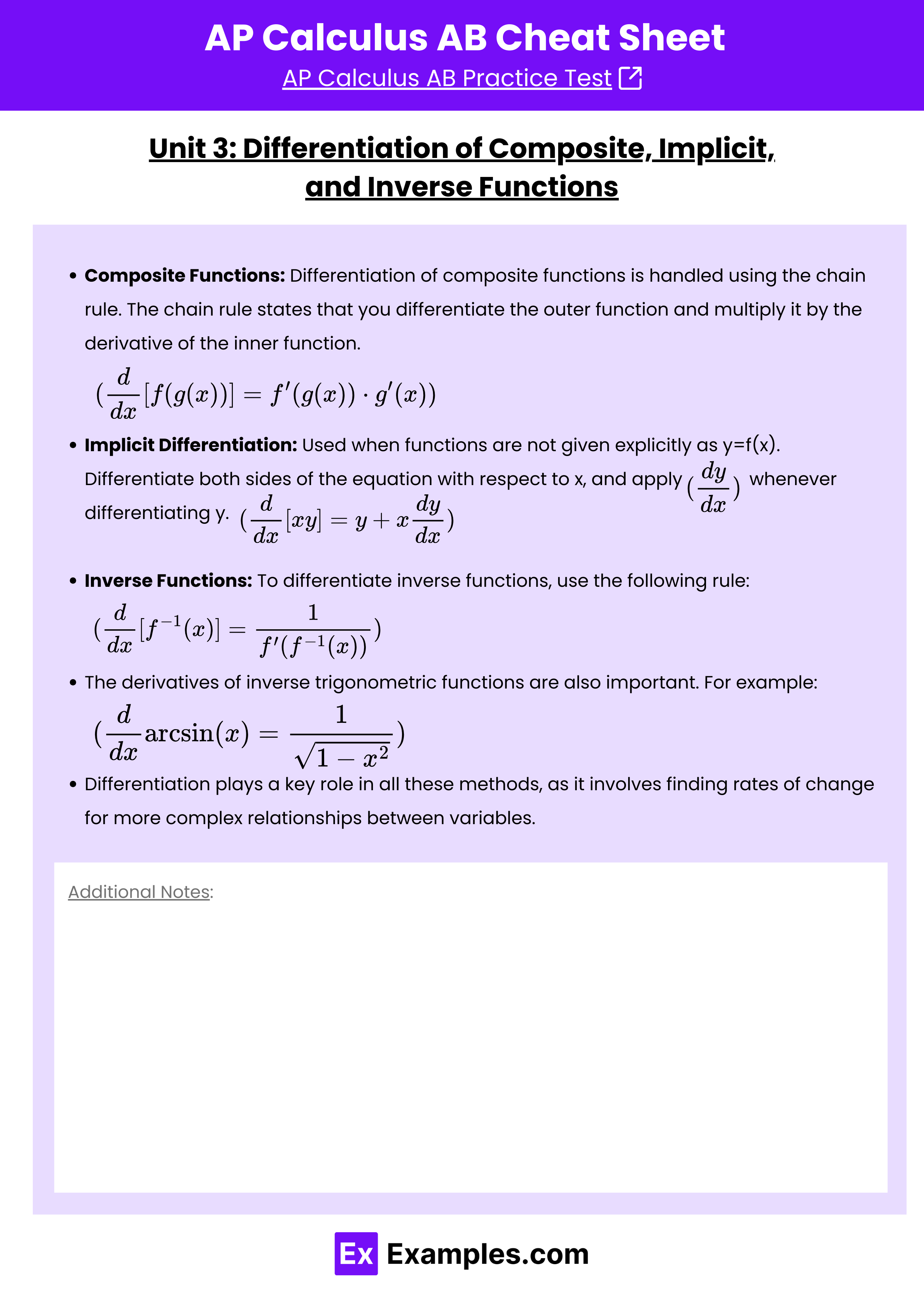
Unit 3: Differentiation of Composite, Implicit, and Inverse Functions

Composite Functions: Differentiation of composite functions is handled using the chain rule. The chain rule states that you differentiate the outer function and multiply it by the derivative of the inner function.

\(\frac{d}{dx} [f(g(x))] = f'(g(x)) \cdot g'(x)\)

Implicit Differentiation: Used when functions are not given explicitly as y=f(x). Differentiate both sides of the equation with respect to x, and apply \(\frac{dy}{dx}\)​ whenever differentiating y.

\(\frac{d}{dx} [xy] = y + x \frac{dy}{dx}\)

Inverse Functions: To differentiate inverse functions, use the following rule:

\(\frac{d}{dx} [f^{-1}(x)] = \frac{1}{f'(f^{-1}(x))}\)

The derivatives of inverse trigonometric functions are also important. For example:

\(\frac{d}{dx} \arcsin(x) = \frac{1}{\sqrt{1 – x^2}}\)

Differentiation plays a key role in all these methods, as it involves finding rates of change for more complex relationships between variables.

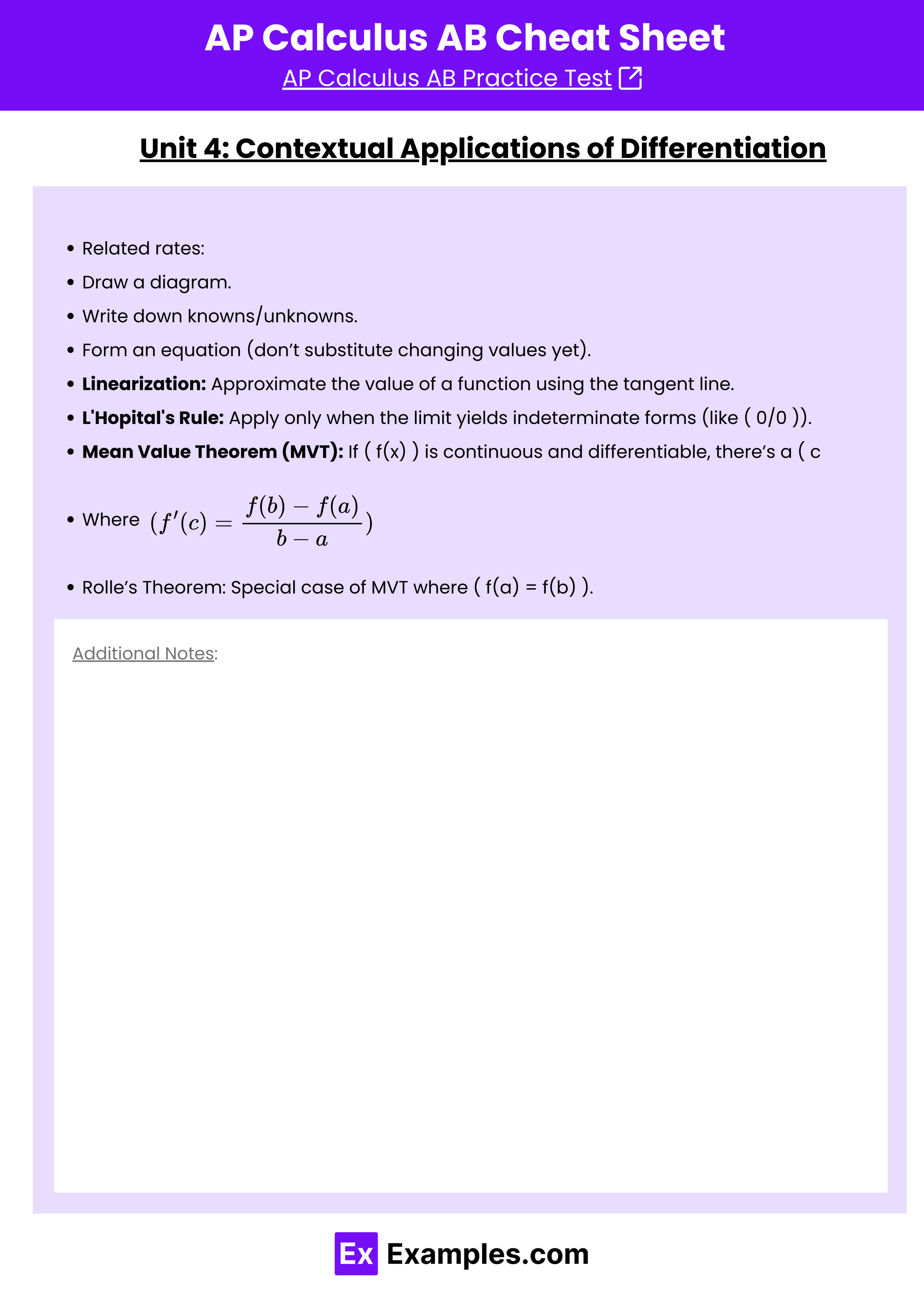
Unit 4: Contextual Applications of Differentiation

• Related rates:

1. Draw a diagram.
2. Write down knowns/unknowns.
3. Form an equation (don’t substitute changing values yet).

• Linearization: Approximate the value of a function using the tangent line.
• L’Hopital’s Rule: Apply only when the limit yields indeterminate forms (like ( 0/0 )).
• Mean Value Theorem (MVT): If ( f(x) ) is continuous and differentiable, there’s a ( c ) Where \(f'(c) = \frac{f(b) – f(a)}{b – a}\)
• Rolle’s Theorem: Special case of MVT where ( f(a) = f(b) ).

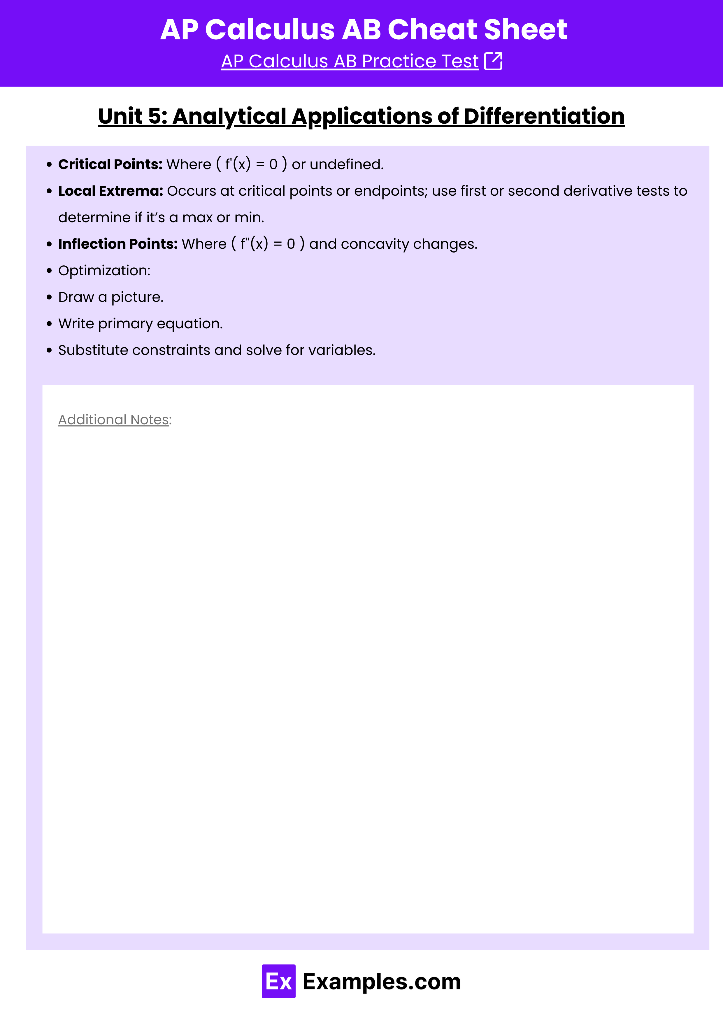
Unit 5: Analytical Applications of Differentiation

• Critical Points: Where ( f'(x) = 0 ) or undefined.
• Local Extrema: Occurs at critical points or endpoints; use first or second derivative tests to determine if it’s a max or min.
• Inflection Points: Where ( f”(x) = 0 ) and concavity changes.
• Optimization:

1. Draw a picture.
2. Write primary equation.
3. Substitute constraints and solve for variables.

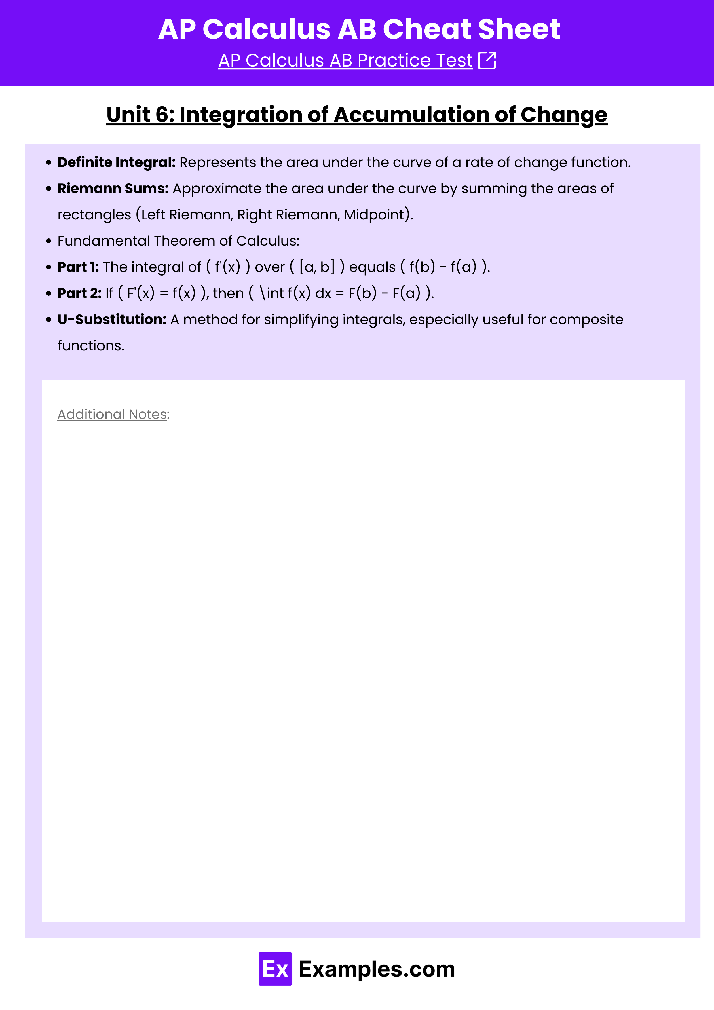
Unit 6: Integration of Accumulation of Change

• Definite Integral: Represents the area under the curve of a rate of change function.
• Riemann Sums: Approximate the area under the curve by summing the areas of rectangles (Left Riemann, Right Riemann, Midpoint).
• Fundamental Theorem of Calculus:
• Part 1: The integral of ( f'(x) ) over ( [a, b] ) equals ( f(b) – f(a) ).
• Part 2: If ( F'(x) = f(x) ), then ( \int f(x) dx = F(b) – F(a) ).
• U-Substitution: A method for simplifying integrals, especially useful for composite functions.

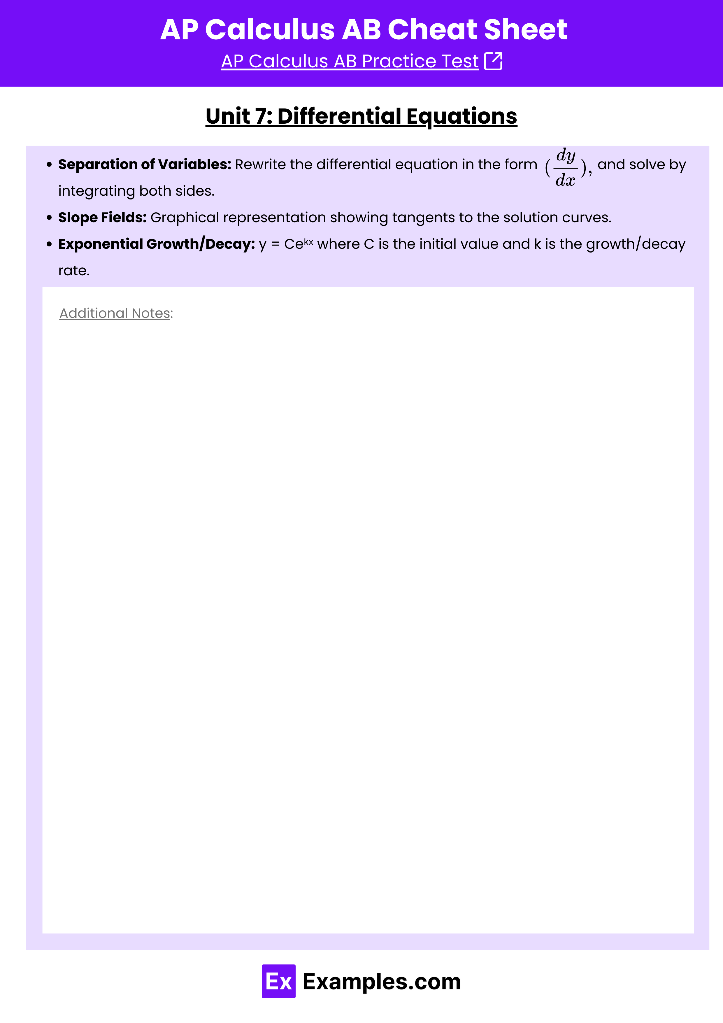
Unit 7: Differential Equations

• Separation of Variables: Rewrite the differential equation in the form \(\frac{dy}{dx}\), and solve by integrating both sides.
• Slope Fields: Graphical representation showing tangents to the solution curves.
• Exponential Growth/Decay: y = Ceᵏˣ where C is the initial value and k is the growth/decay rate.

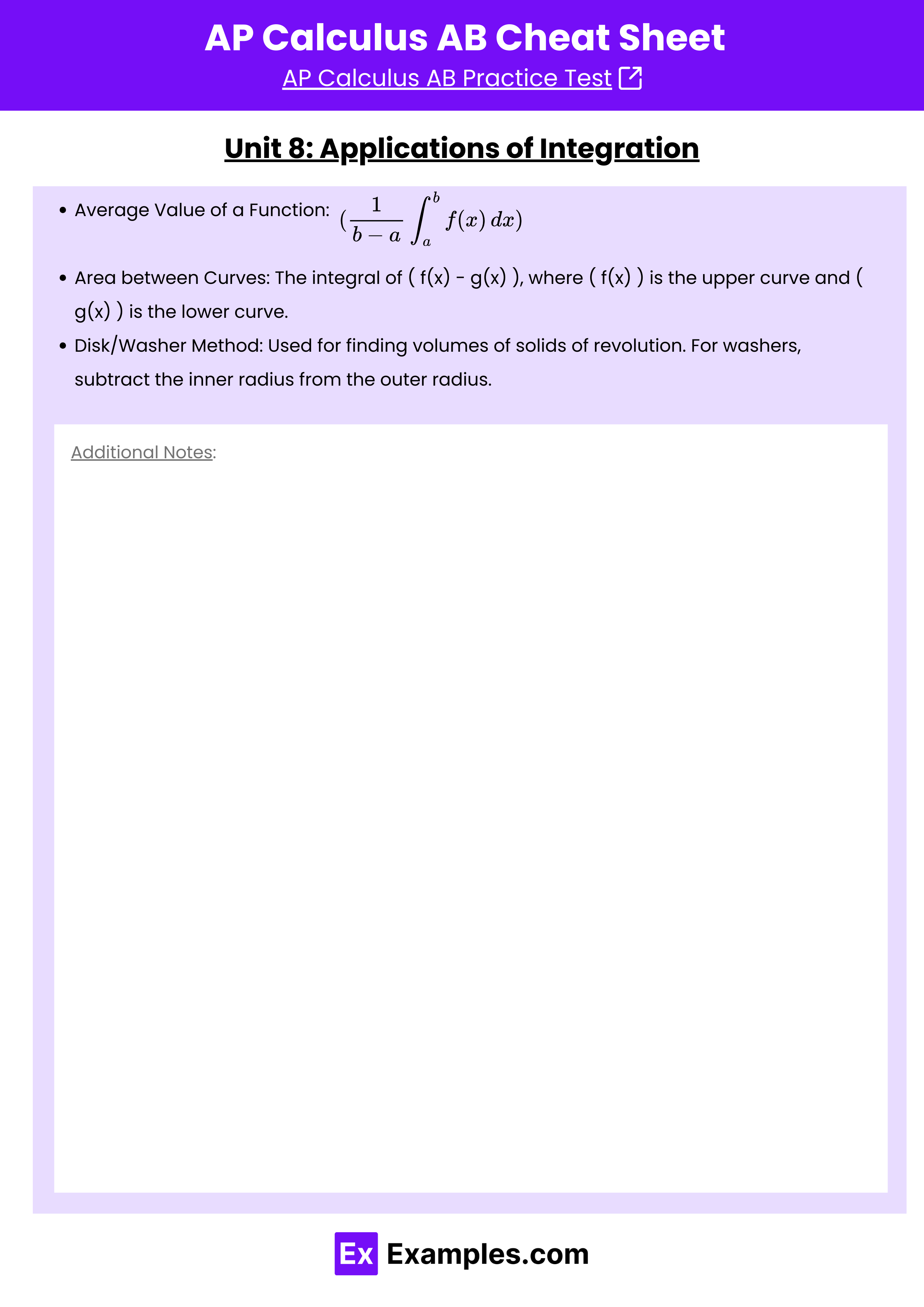
Unit 8: Applications of Integration

• Average Value of a Function: \(\frac{1}{b – a} \int_{a}^{b} f(x)\, dx\)
• Area between Curves: The integral of ( f(x) – g(x) ), where ( f(x) ) is the upper curve and ( g(x) ) is the lower curve.
• Disk/Washer Method: Used for finding volumes of solids of revolution. For washers, subtract the inner radius from the outer radius.