AP® Calculus BC Cheat Sheet

Last Updated: September 23, 2024

Notes

This AP Calculus BC cheat sheet provides a quick reference for key concepts like limits, derivatives, integrals, sequences, series, and parametric equations, helping students prepare efficiently for the AP exam.

Free AP Calculus BC Practice Test

Download AP Calculus BC Cheat sheet – Pdf

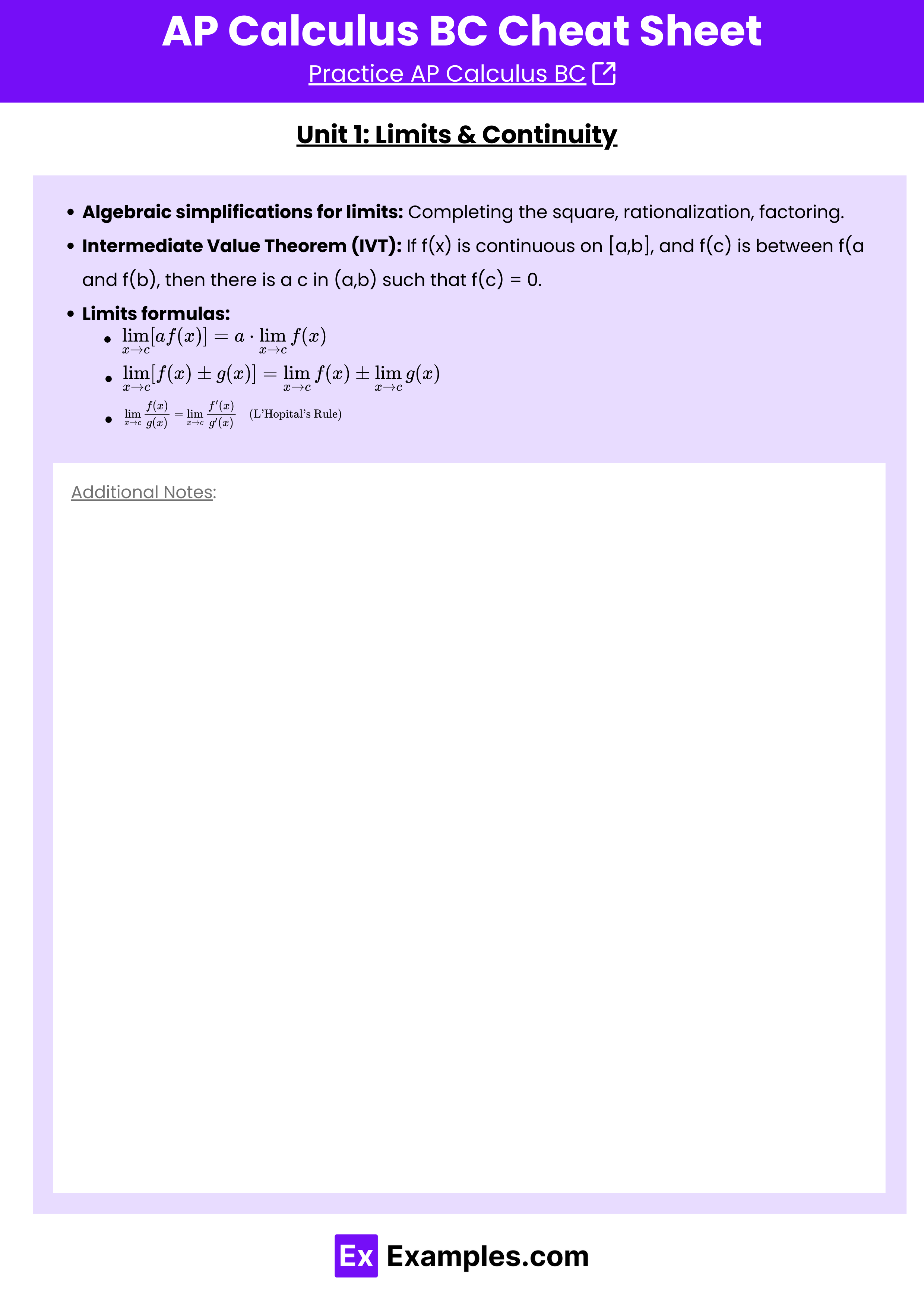
Unit 1: Limits & Continuity

Algebraic simplifications for limits: Completing the square, rationalization, factoring.
Intermediate Value Theorem (IVT): If f(x) is continuous on [a,b], and f(c) is between f(a and f(b), then there is a c in (a,b) such that f(c) = 0.
Limits formulas:
$\lim_{x \to c} [af(x)] = a \cdot \lim_{x \to c} f(x)$
$\lim_{x \to c} [f(x) \pm g(x)] = \lim_{x \to c} f(x) \pm \lim_{x \to c} g(x)$
$\lim_{x \to c} \frac{f(x)}{g(x)} = \lim_{x \to c} \frac{f'(x)}{g'(x)} \quad \text{(L'Hopital's Rule)}$

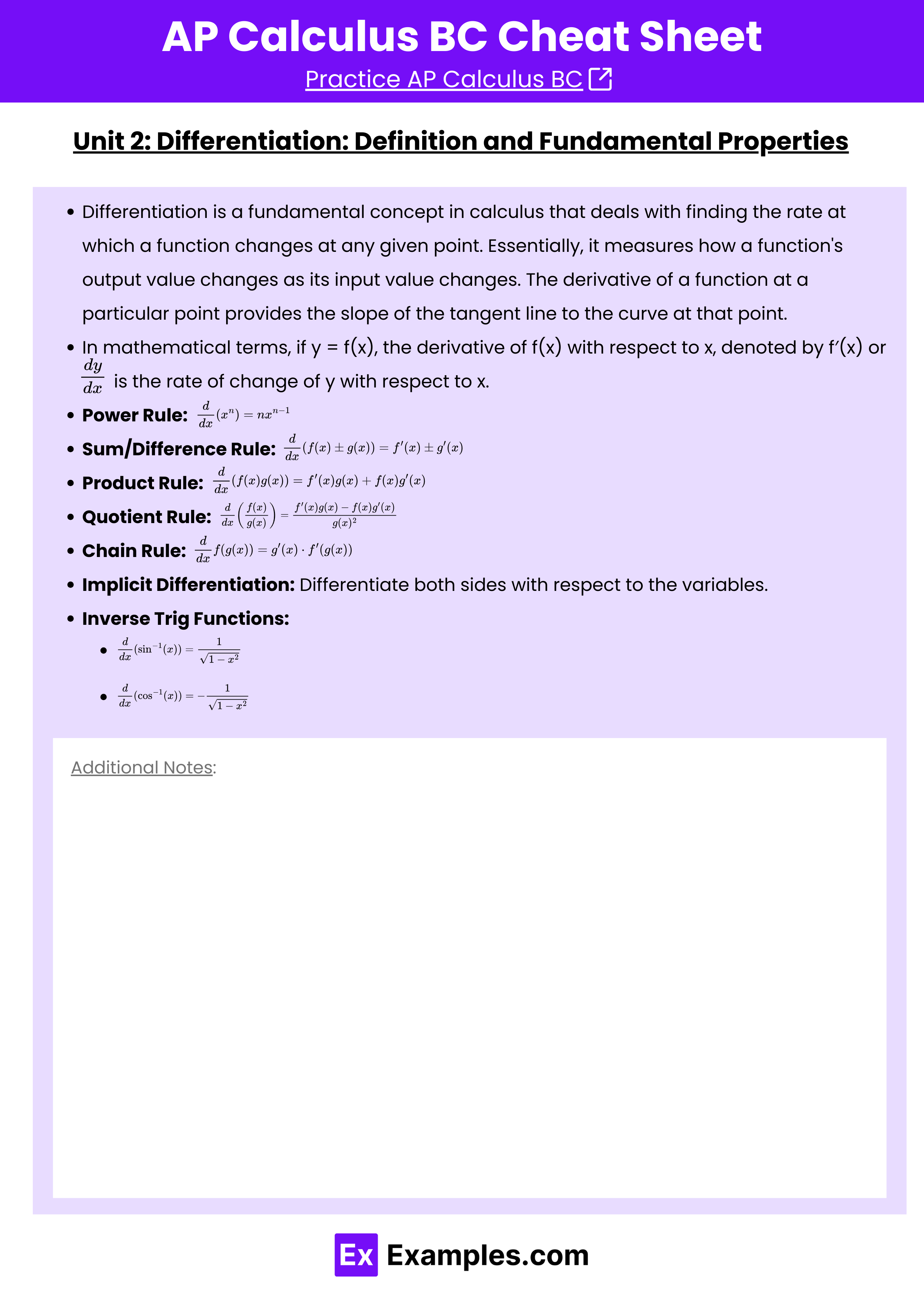
Unit 2: Differentiation: Definition and Fundamental Properties

Differentiation is a fundamental concept in calculus that deals with finding the rate at which a function changes at any given point. Essentially, it measures how a function’s output value changes as its input value changes. The derivative of a function at a particular point provides the slope of the tangent line to the curve at that point.

In mathematical terms, if y = f(x), the derivative of f(x) with respect to x, denoted by f′(x) or $\frac{dy}{dx}$ , is the rate of change of y with respect to x.

Power Rule: $\frac{d}{dx}(x^n) = n x^{n-1}$
Sum/Difference Rule: $\frac{d}{dx}(f(x) \pm g(x)) = f'(x) \pm g'(x)$
Product Rule: $\frac{d}{dx}(f(x)g(x)) = f'(x)g(x) + f(x)g'(x)$
Quotient Rule: $\frac{d}{dx} \left( \frac{f(x)}{g(x)} \right) = \frac{f'(x)g(x) - f(x)g'(x)}{g(x)^2}$
Chain Rule: $\frac{d}{dx} f(g(x)) = g'(x) \cdot f'(g(x))$
Implicit Differentiation: Differentiate both sides with respect to the variables.
Inverse Trig Functions:
$\frac{d}{dx} (\sin^{-1}(x)) = \frac{1}{\sqrt{1 - x^2}}$
$\frac{d}{dx} (\cos^{-1}(x)) = - \frac{1}{\sqrt{1 - x^2}}$

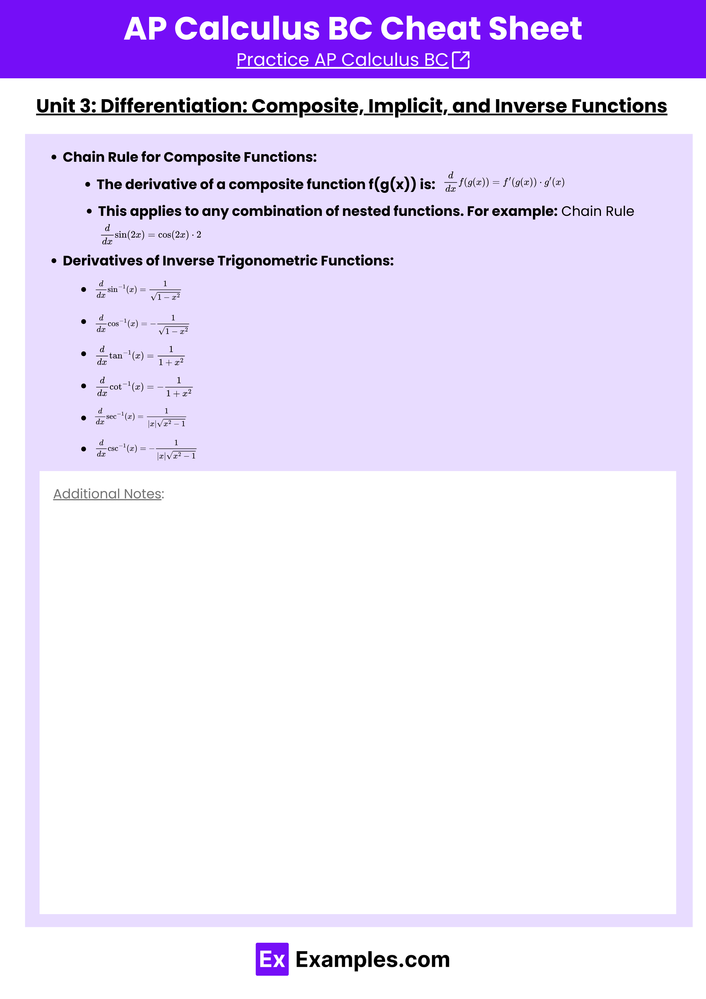
Unit 3: Composite, Implicit, & Inverse Functions

Chain Rule for Composite Functions:

The derivative of a composite function f(g(x)) is: $\frac{d}{dx} f(g(x)) = f'(g(x)) \cdot g'(x)$
This applies to any combination of nested functions. For example: $\frac{d}{dx} \sin(2x) = \cos(2x) \cdot 2$

Derivatives of Inverse Trigonometric Functions:

$\left( f^{-1} \right)'(x) = \frac{1}{f'(f^{-1}(x))}$
$\frac{d}{dx} \sin^{-1}(x) = \frac{1}{\sqrt{1 - x^2}}$
$\frac{d}{dx} \cos^{-1}(x) = -\frac{1}{\sqrt{1 - x^2}}$
$\frac{d}{dx} \tan^{-1}(x) = \frac{1}{1 + x^2}$
$\frac{d}{dx} \cot^{-1}(x) = -\frac{1}{1 + x^2}$
$\frac{d}{dx} \sec^{-1}(x) = \frac{1}{|x| \sqrt{x^2 - 1}}$
$\frac{d}{dx} \csc^{-1}(x) = -\frac{1}{|x| \sqrt{x^2 - 1}}$

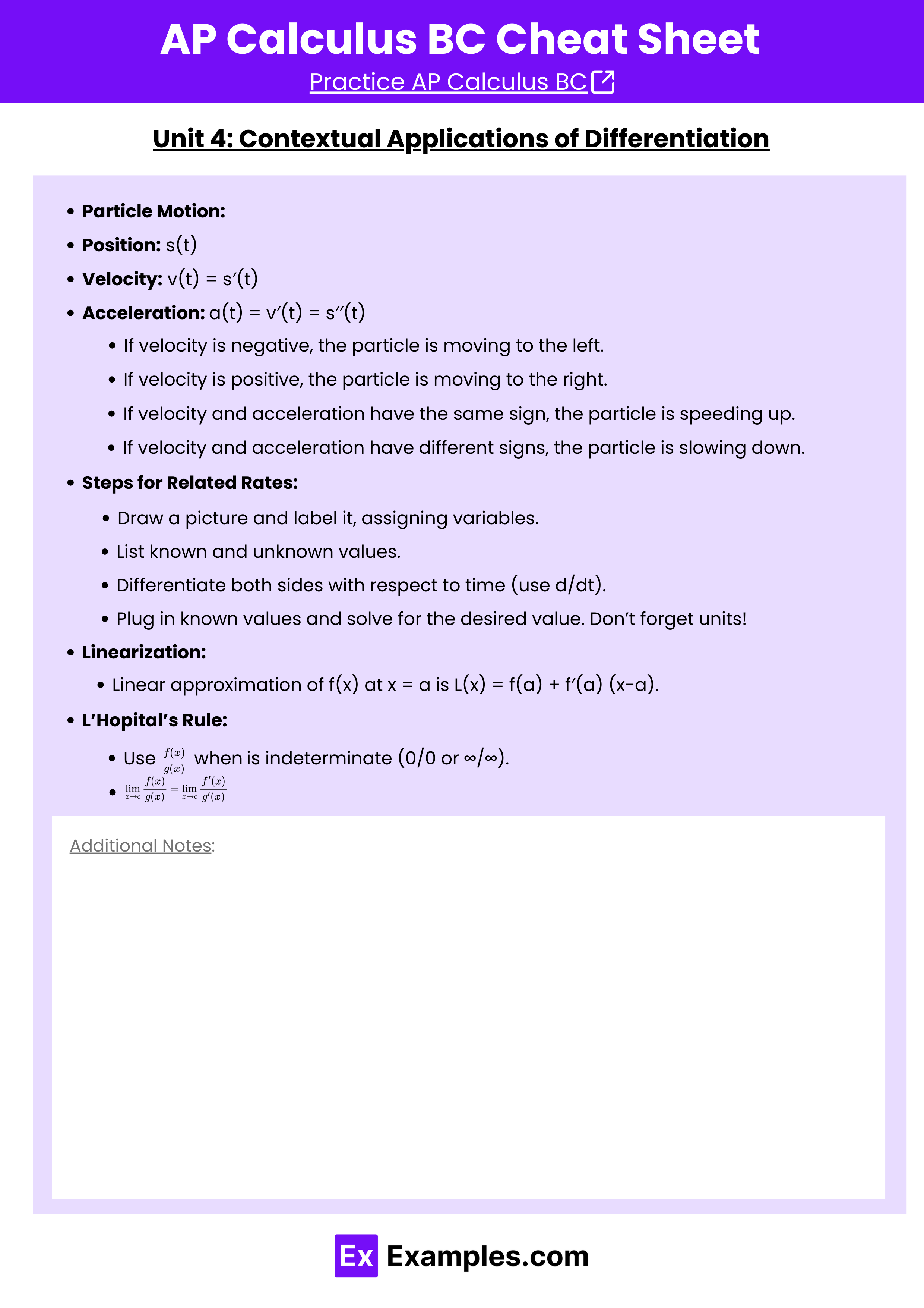
Unit 4: Contextual Applications of Differentiation

Particle Motion:

Position: s(t)
Velocity: v(t) = s′(t)
Acceleration: a(t) = v′(t) = s′′(t)
If velocity is negative, the particle is moving to the left.
If velocity is positive, the particle is moving to the right.
If velocity and acceleration have the same sign, the particle is speeding up.
If velocity and acceleration have different signs, the particle is slowing down.

Steps for Related Rates:

Draw a picture and label it, assigning variables.
List known and unknown values.
Write an equation to model the situation.
Differentiate both sides with respect to time (use d/dt).
Plug in known values and solve for the desired value. Don’t forget units!

Linearization:

Linear approximation of f(x) at x = a is L(x) = f(a) + f′(a) (x−a).

L’Hopital’s Rule:

Use when $\frac{f(x)}{g(x)}$ is indeterminate (0/0 or ∞/∞).
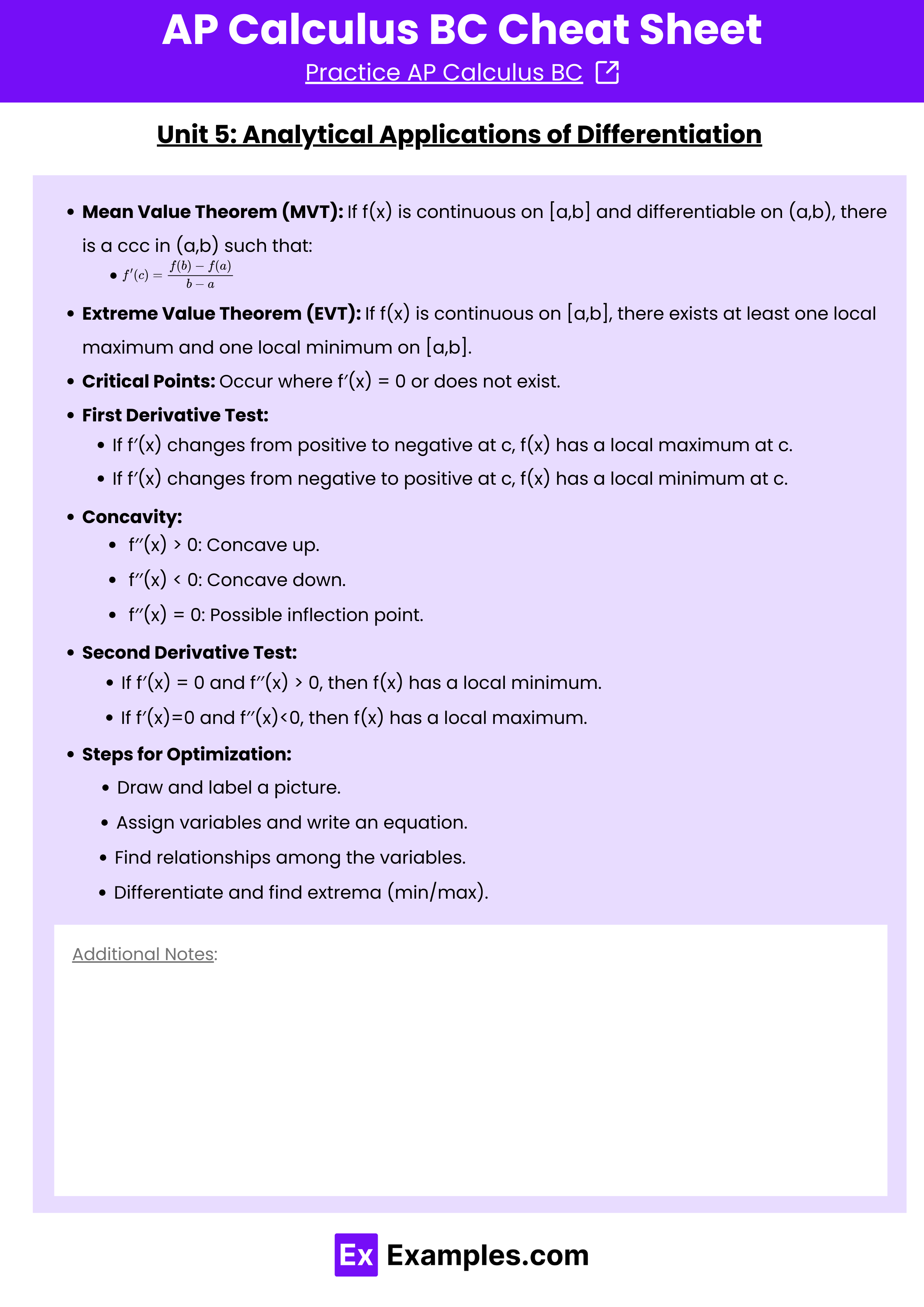
$\lim_{x \to c} \frac{f(x)}{g(x)} = \lim_{x \to c} \frac{f'(x)}{g'(x)}$

Unit 5: Analytical Applications of Differentiation

Mean Value Theorem (MVT):
- If f(x) is continuous on [a,b] and differentiable on (a,b), there is a ccc in (a,b) such that:
Extreme Value Theorem (EVT):
- If f(x) is continuous on [a,b], there exists at least one local maximum and one local minimum on [a,b].
Critical Points:
- Occur where f′(x) = 0 or does not exist.
First Derivative Test:
- If f′(x) changes from positive to negative at c, f(x) has a local maximum at c.
- If f′(x) changes from negative to positive at c, f(x) has a local minimum at c.
Concavity:
- f′′(x) > 0: Concave up.
- f′′(x) < 0: Concave down.
- f′′(x) = 0: Possible inflection point.
Second Derivative Test:
- If f′(x) = 0 and f′′(x) > 0, then f(x) has a local minimum.
- If f′(x)=0 and f′′(x)<0, then f(x) has a local maximum.
Steps for Optimization:
1. Draw and label a picture.
2. Assign variables and write an equation.
3. Find relationships among the variables.
4. Differentiate and find extrema (min/max).

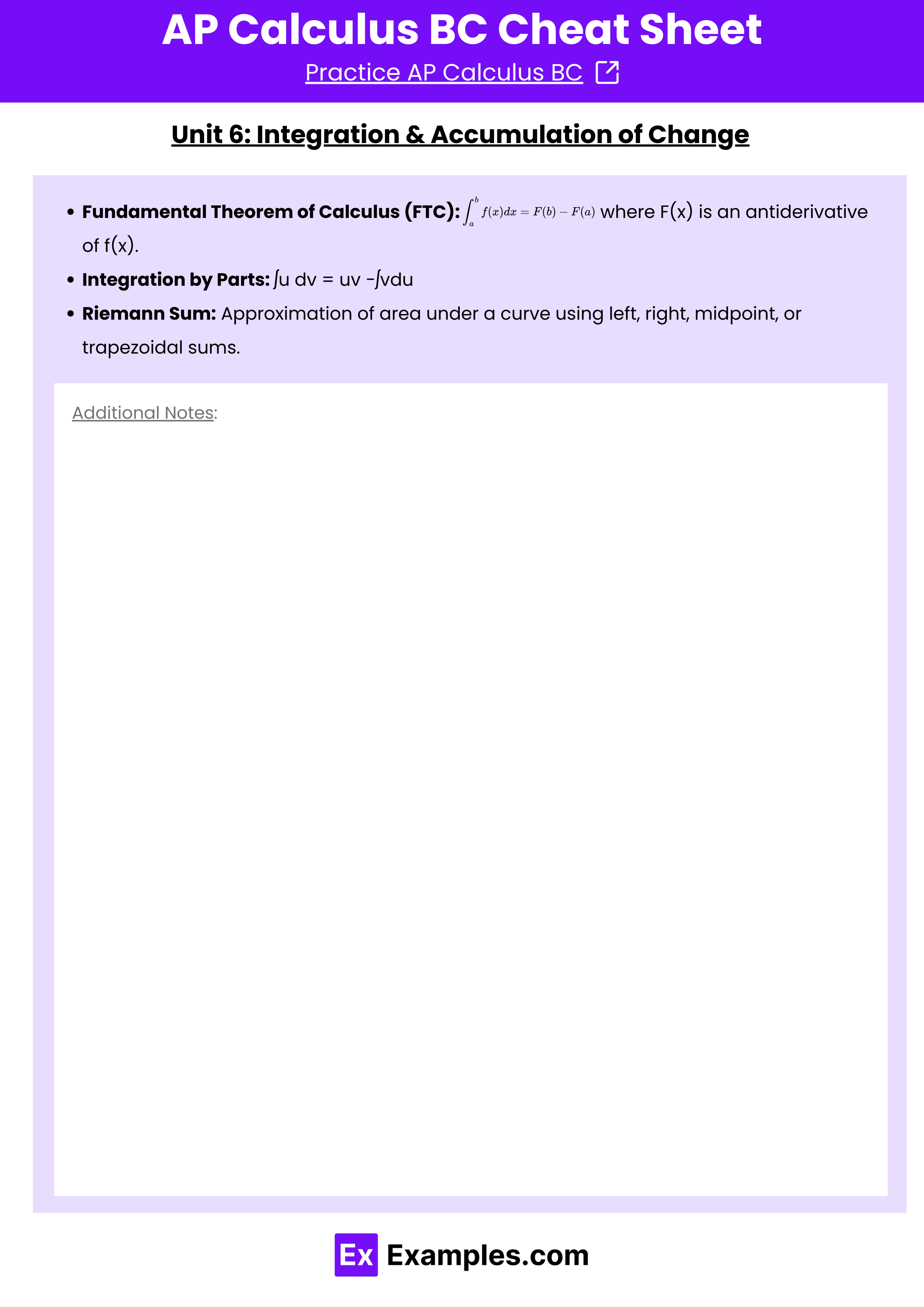
Unit 6: Integration & Accumulation of Change

Fundamental Theorem of Calculus (FTC): $\int_a^b f(x) dx = F(b) - F(a)$ where F(x) is an antiderivative of f(x).
Integration by Parts: ∫u dv = uv −∫vdu
Riemann Sum: Approximation of area under a curve using left, right, midpoint, or trapezoidal sums.

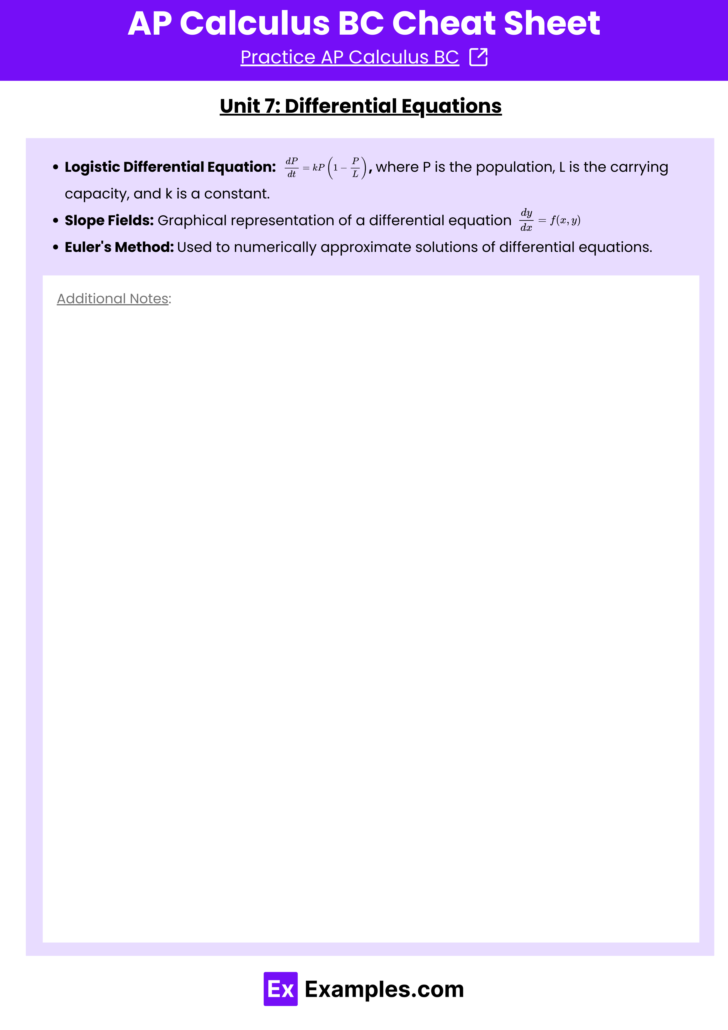
Unit 7: Differential Equations

Logistic Differential Equation: $\frac{dP}{dt} = kP \left( 1 - \frac{P}{L} \right)$ , where P is the population, L is the carrying capacity, and k is a constant.
Slope Fields: Graphical representation of a differential equation $\frac{dy}{dx} = f(x, y)$
Euler’s Method: Used to numerically approximate solutions of differential equations.

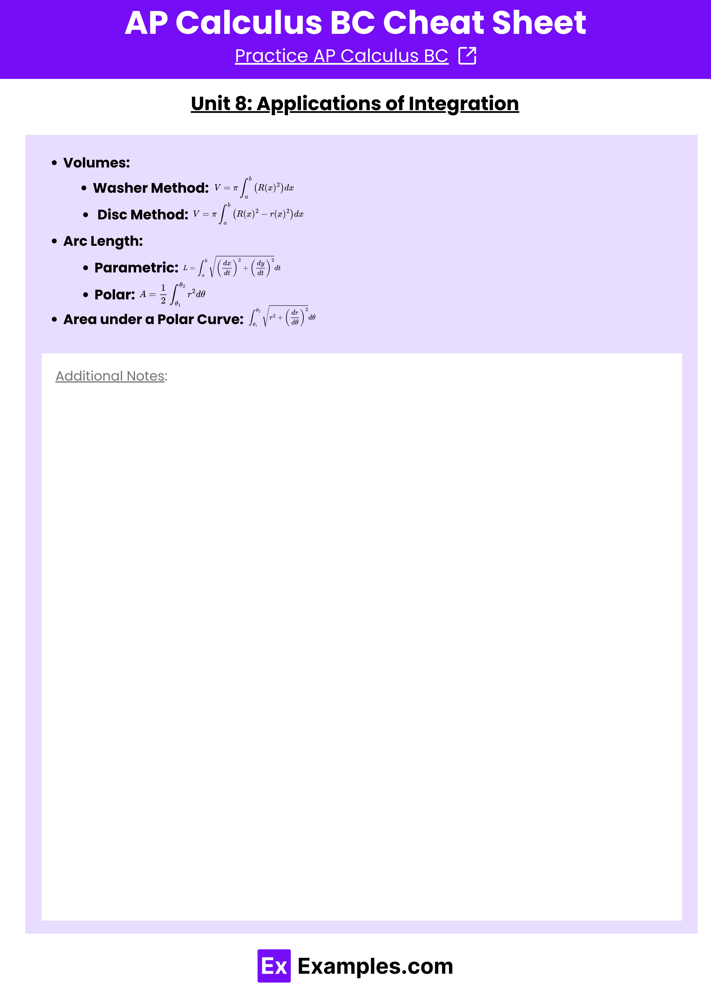
Unit 8: Applications of Integration

Volumes:

Washer Method: $V = \pi \int_a^b \left( R(x)^2 - r(x)^2 \right) dx$
Disc Method: $V = \pi \int_a^b \left( R(x)^2 \right) dx$

Arc Length:

Parametric: $L = \int_a^b \sqrt{\left( \frac{dx}{dt} \right)^2 + \left( \frac{dy}{dt} \right)^2} dt$
Polar:

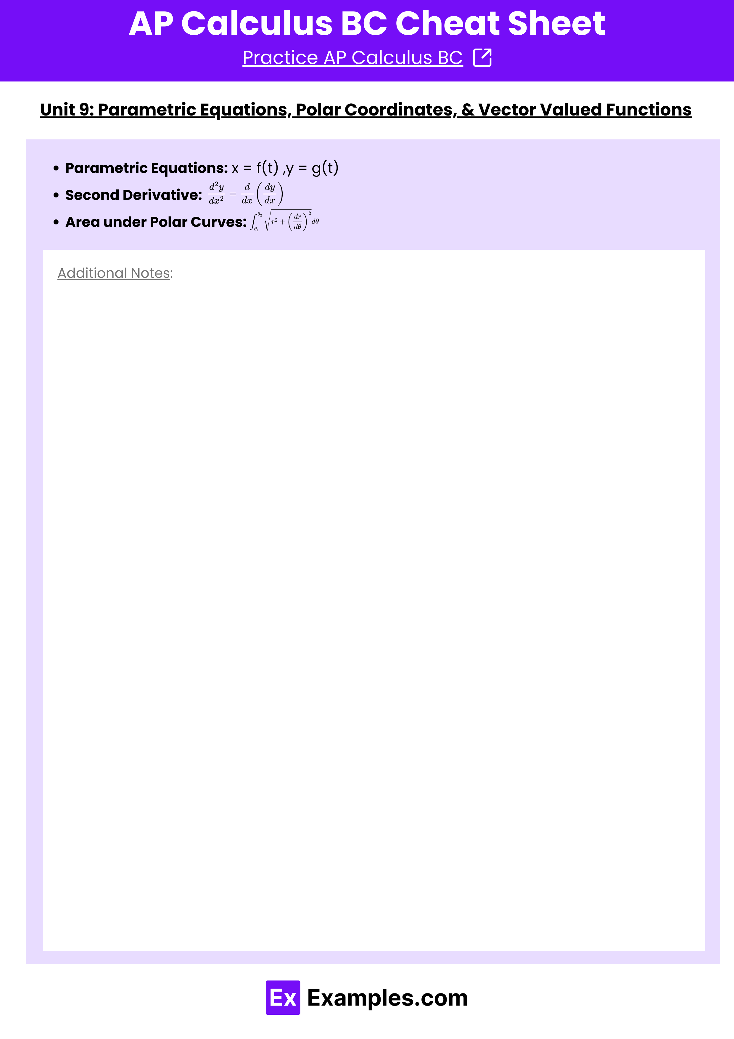
Unit 9: Parametric Equations, Polar Coordinates, and Vector-Valued Functions
- Parametric Equations: x = f(t) ,y = g(t)
- Second Derivative: $\frac{d^2 y}{dx^2} = \frac{d}{dx} \left( \frac{dy}{dx} \right)$
- Area under Polar Curves: $A = \frac{1}{2} \int_{\theta_1}^{\theta_2} r^2 d\theta$
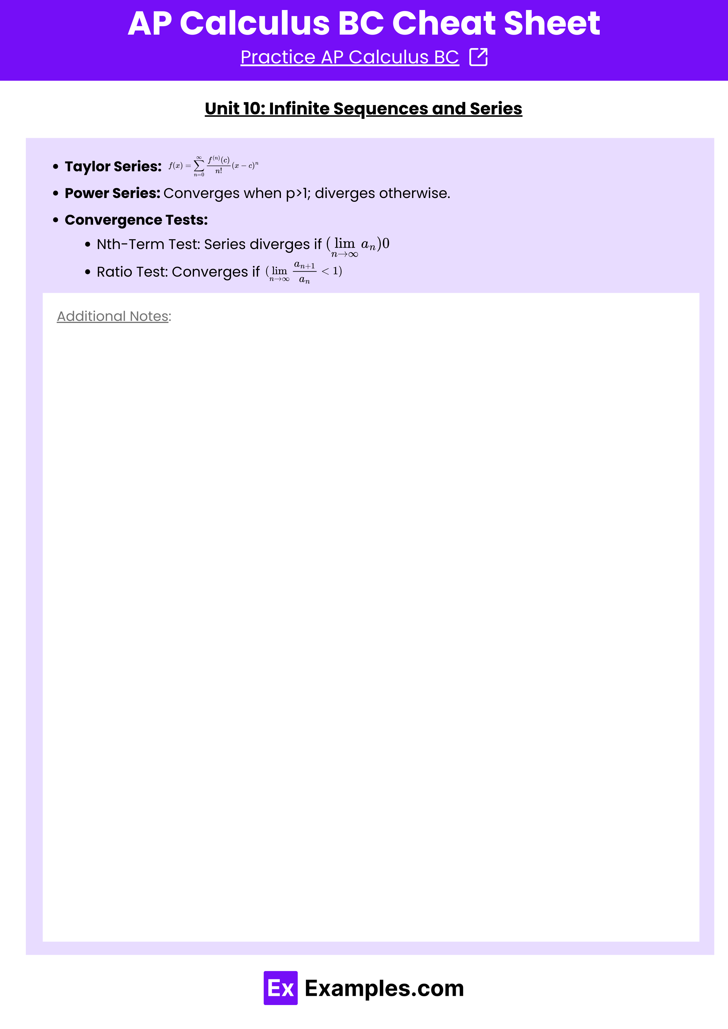
Unit 10: Infinite Sequences and Series

Taylor Series:
- $f(x) = \sum_{n=0}^{\infty} \frac{f^{(n)}(c)}{n!}(x - c)^n$
Power Series: Converges when p>1; diverges otherwise.

Convergence Tests:
- Nth-Term Test: Series diverges if $\lim_{n \to \infty} a_n$ 0
- Ratio Test: Converges if $\lim_{n \to \infty} \frac{a_{n+1}}{a_n} < 1$