Approximating Integrals Using Riemann Sums

In AP Calculus AB and BC, approximating integrals using Riemann sums is a foundational technique for estimating the area under a curve. By dividing an interval into smaller subintervals, Riemann sums calculate the sum of rectangular areas that approximate the definite integral. This method helps students understand the concept of integration and its applications, such as finding total distance traveled or the accumulated value of a function. Riemann sums are essential for grasping the transition from discrete sums to continuous integration.

Learning Objectives

For the AP Calculus AB and BC exams, you should focus on mastering how to approximate the value of definite integrals using Riemann sums. This includes understanding and applying left, right, and midpoint Riemann sums to estimate areas under curves. You should also learn to divide intervals, calculate subinterval widths, and evaluate functions at specific points. Additionally, be familiar with the concepts of increasing the number of subintervals to improve accuracy and comparing these approximations to the exact integral values.

Introduction to Riemann Sums

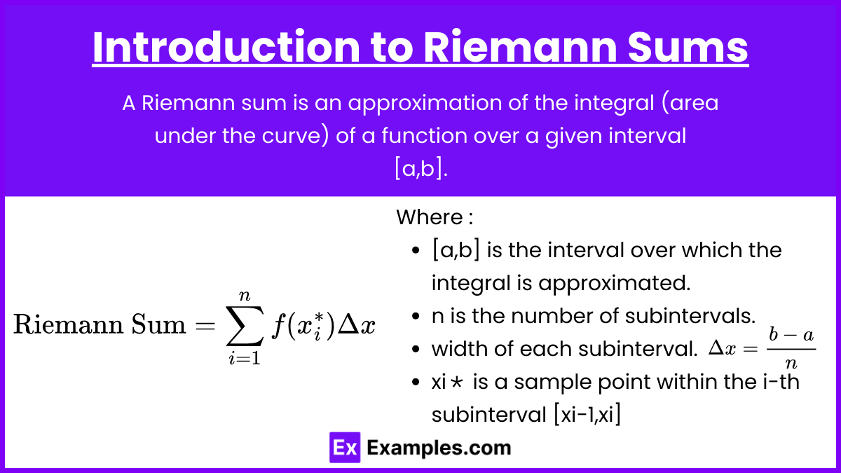
A Riemann sum is an approximation of the integral (area under the curve) of a function over a given interval
[a,b]. It is calculated by dividing the interval into smaller subintervals, calculating the function’s value at specific points within those subintervals, and summing up the areas of the rectangles formed.

Riemann Sums are used to approximate the value of a definite integral. The idea is to partition the interval over which the function is defined into smaller subintervals, calculate the function’s value at specific points within these subintervals, multiply these values by the width of the subintervals, and sum the results.

Given a continuous function f(x) on the interval [a,b], a Riemann sum is given by:

\(\text{Riemann Sum} = \sum_{i=1}^{n} f(x_i^*) \Delta x \)

Where:

• [a,b] is the interval over which the integral is approximated.
• n is the number of subintervals.
• \( \Delta x = \frac{b-a}{n} \) is the width of each subinterval.
• \( x_i^* \) is a sample point within the i-th subinterval [x_i−1,x_i], chosen based on the type of Riemann sum.

Types of Riemann Sums

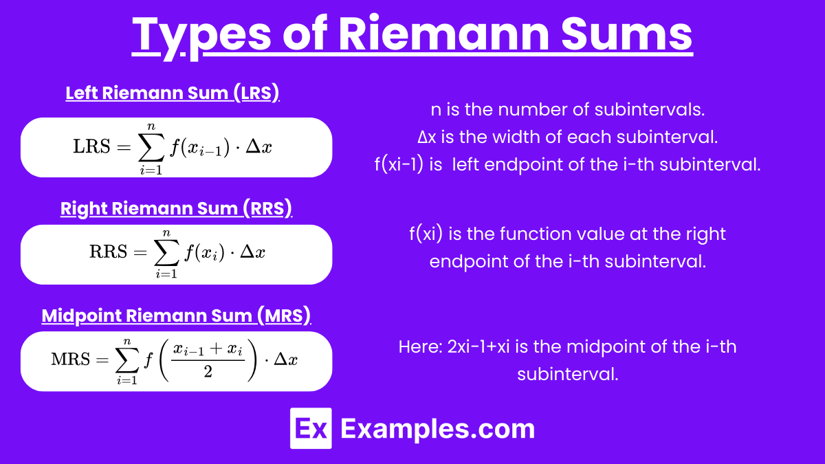
There are three main types of Riemann Sums:

• Left Riemann Sum (LRS)
• Right Riemann Sum (RRS)
• Midpoint Riemann Sum (MRS)

Left Riemann Sum (LRS)

In the Left Riemann Sum, the height of each rectangle is determined by the function’s value at the left endpoint of each subinterval.

Formula:

\(\text{LRS} = \sum_{i=1}^{n} f(x_{i-1}) \cdot \Delta x \)

Here:

• n is the number of subintervals.
• Δx is the width of each subinterval.
• f(x_i−1​) is the function value at the left endpoint of the i-th subinterval.

Right Riemann Sum (RRS)

In the Right Riemann Sum, the height of each rectangle is determined by the function’s value at the right endpoint of each subinterval.

Formula:

\(\text{RRS} = \sum_{i=1}^{n} f(x_i) \cdot \Delta x \)

Here:

• f(x_i​) is the function value at the right endpoint of the i-th subinterval.

Midpoint Riemann Sum (MRS)

In the Midpoint Riemann Sum, the height of each rectangle is determined by the function’s value at the midpoint of each subinterval.

Formula:

\(\text{MRS} = \sum_{i=1}^{n} f\left(\frac{x_{i-1} + x_i}{2}\right) \cdot \Delta x \)

Here: 2x_i−1​+x_i​​ is the midpoint of the i-th subinterval.

Steps to Approximate Integrals Using Riemann Sums

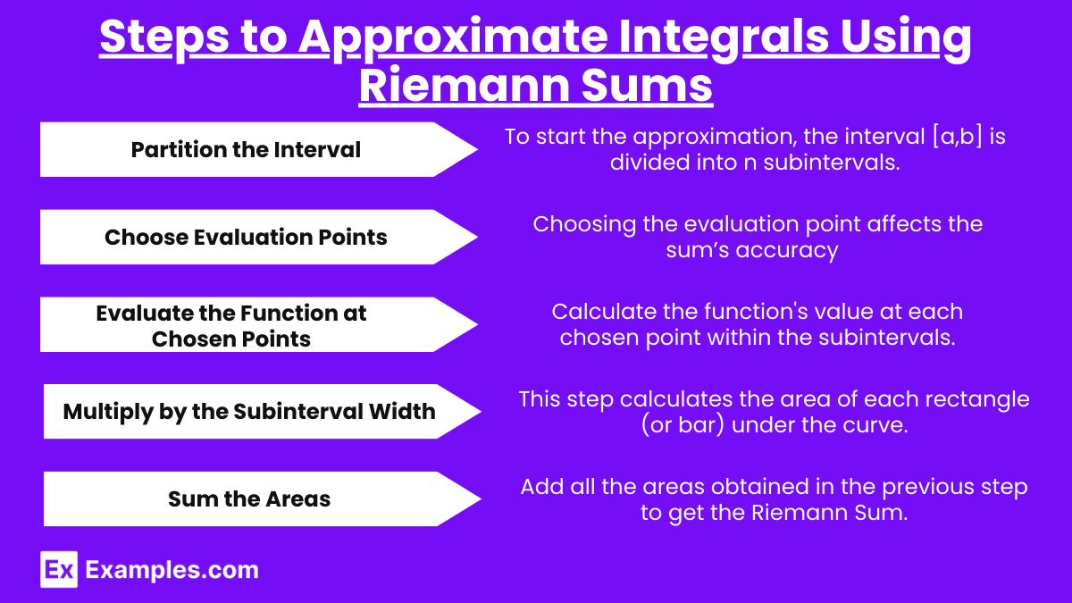
Step 1: Partition the Interval

• To start the approximation, the interval [a,b] is divided into n subintervals.
• The interval [a,b] is divided into n subintervals.
• The width of each subinterval is \( \Delta x = \frac{b – a}{n} \)​.
• Increasing the number of subintervals n improves the approximation because the rectangles used in the Riemann Sum will more closely fit the curve.

Step 2: Choose Evaluation Points

• For LRS: Use the left endpoint of each subinterval.
• For RRS: Use the right endpoint of each subinterval.
• For MRS: Use the midpoint of each subinterval. Choosing the evaluation point affects the sum’s accuracy and how well it approximates the actual area under the curve.

Step 3: Evaluate the Function at Chosen Points

• Calculate the function’s value at each chosen point within the subintervals.
• This step determines the height of the rectangle corresponding to each subinterval, which will be used to approximate the area under the curve over that subinterval.

Step 4: Multiply by the Subinterval Width

• After evaluating the function at the chosen points, multiply each function value by the width of the subinterval, Δx.
• This step calculates the area of each rectangle (or bar) under the curve.

Step 5: Sum the Areas

• Finally, sum the areas of all the rectangles to obtain the Riemann Sum, which approximates the value of the definite integral over [a,b]
• Add all the areas obtained in the previous step to get the Riemann Sum.

Examples

Example 1. Left Riemann Sum for y = x² on [0, 2]

Divide [0,2] into 4 intervals, each of width Δx = 0.5. Use left endpoints to find function values: f(0) = 0, f(0.5) = 0.25, f(1) = 1, and f(1.5) = 2.25. The approximate area is 0.5 (0+0.25+1+2.25) = 1.75.

Example 2. Right Riemann Sum for y = sin(x) on [0, π]

Divide [0,π] into 3 intervals, each of width \( \Delta x = \frac{\pi}{3} \)​. Use right endpoints: \( \sin\left(\frac{\pi}{3}\right) \), \( \sin\left(\frac{2\pi}{3}\right) \), and \( \sin(\pi) \). The sum is \( \frac{\pi}{3}\left(\frac{\sqrt{3}}{2} + \frac{\sqrt{3}}{2} + 0\right) \).

Example 3. Midpoint Riemann Sum for y = e^x on [0, 1]

Divide [0,1] into 2 intervals of width Δx = 0.5. Use midpoints f(0.25) = e^0.25 and f(0.75) = e^0.75. The sum is 0.5(e0.25+e0.75).

Example 4. Left Riemann Sum for y=1/x on [1, 3]

Divide [1,3] into 4 intervals of width Δx=0.5. Use left endpoints: f(1)=1, f(1.5)=32​, f(2)=0.5, f(2.5)=0.4. The sum is \( 0.5\left(e^{0.25} + e^{0.75}\right) \).

Example 5. Right Riemann Sum for y = cos(x) on \([0, \frac{\pi}{2}]\)

Divide \([0, \frac{\pi}{2}]\) into 2 intervals of width \( \Delta x = \frac{\pi}{4} \). Use right endpoints: \( \cos\left(\frac{\pi}{4}\right) = \frac{\sqrt{2}}{2} \) and \( \cos\left(\frac{\pi}{2}\right) = 0 \). The sum is \( \frac{\pi}{4}\left(\frac{\sqrt{2}}{2} + 0\right) \).

Multiple Choice Questions

Question 1

Given the function f(x) = 3x² on the interval [1,4], which of the following represents the width Δx of each subinterval if the interval is divided into 6 subintervals?

A) Δx = 0.5
B) Δx = 1.5
C) Δx = 2.0
D) Δx = 0.75

Answer: D) Δx = 0.5

Explanation: To find the width of each subinterval, use the formula:

\( \Delta x = \frac{b – a}{n} \)

Here, a = 1, b = 4, and n = 6.

Δx = 4−1​/6 = 3/6 ​= 0.5

So, the correct answer is Δx = 0.5.

Question 2

Consider the function f(x) = x+2 on the interval [0,2]. Using the Right Riemann Sum with 4 subintervals, which of the following is the correct approximation of the integral \( \int_{0}^{2} (x + 2) \, dx \)?

A) 8.5
B) 10.5
C) 9.0
D) 8.0

Answer: A) 8.5

Explanation: First, calculate the width of each subinterval:

Δx = 2−0/4 ​ = 2/4 = 0.5

Next, find the right endpoints of each subinterval:

• Right points: x₁​ = 0.5, x₂​ = 1.0, x₃ ​= 1.5, x₄​ = 2.0

Evaluate the function at these points:

f(0.5) = 0.5 + 2 = 2.5
f(1.0) = 1.0 + 2 = 3.0
f(1.5) = 1.5 + 2 = 3.5
f(2.0) = 2.0 + 2 = 4.0

Now, calculate the Right Riemann

\( \text{RRS} = \sum_{i=1}^{4} f(x_i) \cdot \Delta x = (2.5 \times 0.5) + (3.0 \times 0.5) + (3.5 \times 0.5) + (4.0 \times 0.5) \)

\( \text{RRS} = 1.25 + 1.5 + 1.75 + 2.0 = 6.5 \)

The correct approximation is 6.5, so the correct answer is A) 6.5.

Question 3

For the function f(x) = x² on the interval [2,3], which type of Riemann Sum typically provides the most accurate approximation of the integral when using the same number of subintervals?

A) Left Riemann Sum
B) Right Riemann Sum
C) Midpoint Riemann Sum
D) All are equally accurate

Answer: C) Midpoint Riemann Sum

Explanation: The Midpoint Riemann Sum generally provides a more accurate approximation than the Left or Right Riemann Sums because it evaluates the function at the midpoint of each subinterval, which often gives a better representation of the average value of the function over the subinterval. This is particularly true for functions that are increasing or decreasing consistently over an interval, as the midpoint can better capture the overall behavior of the function within each subinterval.

Therefore, the correct answer is C) Midpoint Riemann Sum.

These questions and explanations are designed to help reinforce the concepts of Riemann Sums, how they are calculated, and which method typically yields a more accurate approximation. They are aimed at building a foundational understanding for students preparing for the AP Calculus exam.