Defining the Derivative of a Function at a Point and as a Function

The derivative is a fundamental concept in calculus, central to both AP Calculus AB and BC. It measures how a function changes as its input changes, providing insights into the function’s behavior. The derivative can be defined at a specific point, where it represents the slope of the tangent line to the curve, and as a function, which describes the rate of change across the entire domain. Mastery of derivatives is crucial for solving problems related to rates of change, optimization, and motion.

Learning Objectives

By studying “Defining the Derivative of a Function at a Point and as a Function,” you should learn to precisely calculate the derivative at a specific point using the limit definition, interpret it as the slope of the tangent line, and generalize this to understand the derivative as a function across its domain. You’ll also master applying derivative rules (power, product, quotient, chain) and explore higher-order derivatives for analyzing concavity and optimization. These skills are crucial for excelling in both AP Calculus AB and BC.

The Derivative of a Function at a Point

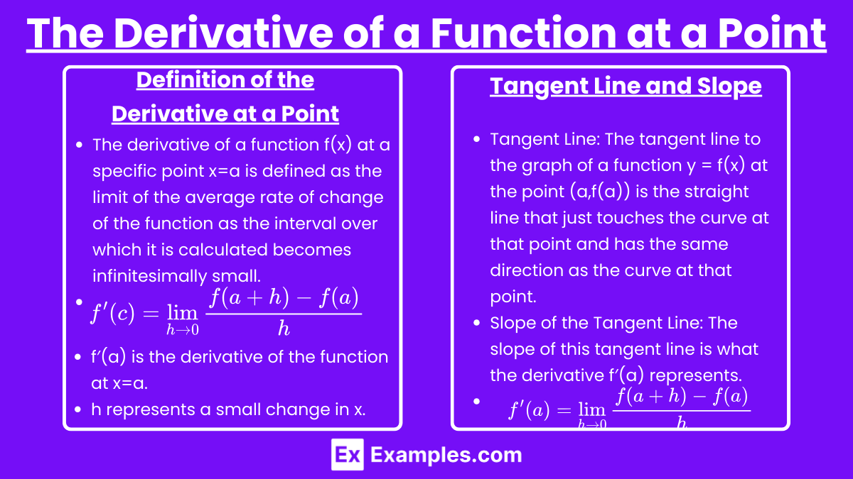
Definition of the Derivative at a Point : The derivative of a function f(x) at a specific point x=a is defined as the limit of the average rate of change of the function as the interval over which it is calculated becomes infinitesimally small. Mathematically, this is expressed as:

\( f'(c) = \lim_{h \to 0} \frac{f(a + h) – f(a)}{h} \)

Here:

f′(a) is the derivative of the function at x=a.
h represents a small change in x.
f(a+h)−f(a) is the change in the function’s value corresponding to the change in x.

Geometric Interpretation : Geometrically, the derivative at a point represents the slope of the tangent line to the graph of the function at that point. If you imagine zooming in on the curve at x=a, the curve becomes almost a straight line, and the slope of this line is f′(a).

Tangent Line and Slope

Tangent Line: The tangent line to the graph of a function y = f(x) at the point (a,f(a)) is the straight line that just touches the curve at that point and has the same direction as the curve at that point. This line does not cross the curve near x=a but just “hugs” the curve at that specific point.
Slope of the Tangent Line: The slope of this tangent line is what the derivative f′(a) represents. Mathematically, this slope is given by the limit of the difference quotient:
\( f'(a) = \lim_{h \to 0} \frac{f(a + h) – f(a)}{h} \)

As h approaches zero, the secant line (the line connecting (a,f(a)) and (a+h,f(a+h))) becomes the tangent line.

The Derivative of a Function as a Function

Definition of the Derivative as a Function

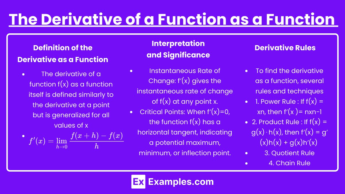
The derivative of a function f(x) as a function itself is defined similarly to the derivative at a point but is generalized for all values of x:

\( f'(x) = \lim_{h \to 0} \frac{f(x + h) – f(x)}{h} \)

This expression provides a new function f′(x) that gives the slope of the tangent line to the graph of f(x) at any point x.

Interpretation and Significance

Instantaneous Rate of Change: f′(x) gives the instantaneous rate of change of f(x) at any point x.
Critical Points: When f′(x)=0, the function f(x) has a horizontal tangent, indicating a potential maximum, minimum, or inflection point.

Derivative Rules

To find the derivative as a function, several rules and techniques are often used:

Power Rule: If f(x) = xⁿ, then f′(x )= nxⁿ⁻¹.
Product Rule: If f(x) = g(x)⋅h(x), then f′(x) = g′(x)h(x) + g(x)h′(x).
Quotient Rule: If f(x) = g(x) h(x), then \( f'(x) = \frac{g'(x)h(x) – g(x)h'(x)}{(h(x))^2} \).
Chain Rule: If f(x) = g(h(x)), then f′(x) = g′(h(x))⋅h′(x).

Connections Between the Derivative at a Point and as a Function

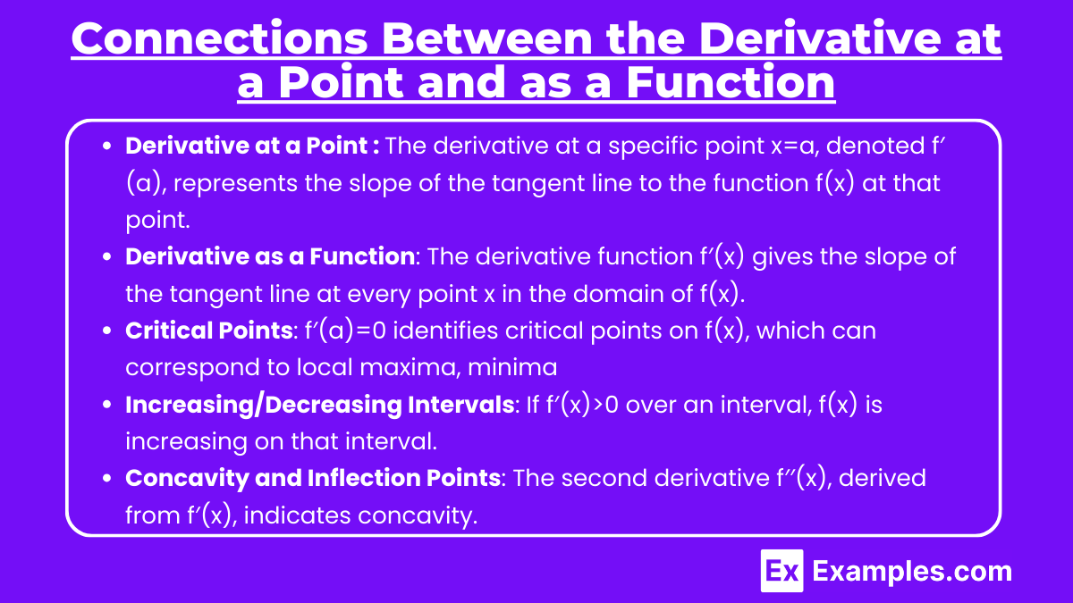
Derivative at a Point: The derivative at a specific point x=a, denoted f′(a), represents the slope of the tangent line to the function f(x) at that point. It provides the instantaneous rate of change of the function at x=a.
Derivative as a Function: The derivative function f′(x) gives the slope of the tangent line at every point x in the domain of f(x). It describes how the rate of change varies across the entire function.
Critical Points: f′(a)=0 identifies critical points on f(x), which can correspond to local maxima, minima, or inflection points, depending on the behavior of f′(x) around x=a.
Increasing/Decreasing Intervals: If f′(x)>0 over an interval, f(x) is increasing on that interval. If f′(x)<0, f(x) is decreasing.
Concavity and Inflection Points: The second derivative f′′(x), derived from f′(x), indicates concavity. Changes in concavity at points where f′′(x)=0 reveal inflection points on f(x).

Higher-Order Derivatives (AP Calculus BC)

While AP Calculus AB focuses on the first derivative, AP Calculus BC also explores higher-order derivatives, such as the second derivative, which is the derivative of the derivative function f′′(x) = d²f / dx². The second derivative provides information about the concavity of the original function and is crucial in analyzing the curvature of graphs.

Given f(x) = 3x³−5x²+2x−4, find the second derivative: f′(x) = 9x²−10x+2

f′′(x) = d/dx (9x²−10x+2) = 18x−10

The second derivative f′′(x)=18x−10 gives information about the concavity of the graph of f(x).

Application of Derivatives

Understanding derivatives is essential for various applications:

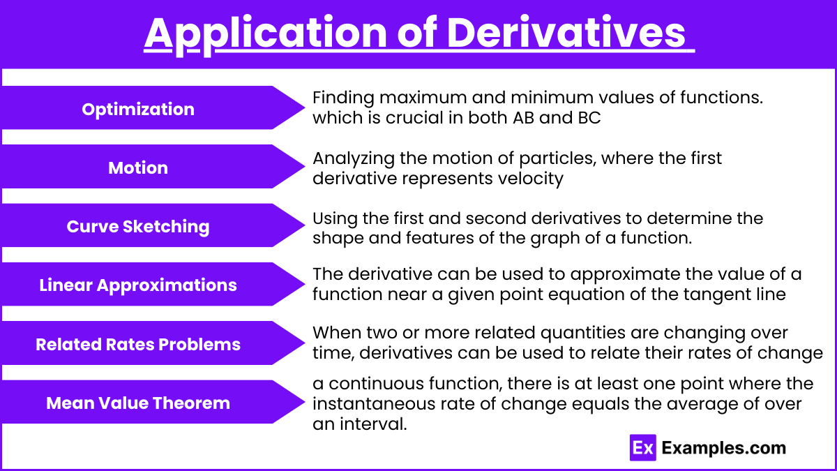
Optimization: Finding maximum and minimum values of functions, which is crucial in both AB and BC.
Motion: Analyzing the motion of particles, where the first derivative represents velocity and the second derivative represents acceleration.
Curve Sketching: Using the first and second derivatives to determine the shape and features of the graph of a function.
Linear Approximations and Differentials:The derivative can be used to approximate the value of a function near a given point using the equation of the tangent line. This is particularly useful for estimating values of complicated functions without needing to compute the exact value. In calculus, differentials help approximate small changes in a function’s value based on changes in the input, providing a practical application in engineering and physics.
Related Rates Problems : Interrelated Quantities: When two or more related quantities are changing over time, derivatives can be used to relate their rates of change. This is crucial in physics, chemistry, and economics, where variables are often interdependent.
Mean Value Theorem : Connecting Average and Instantaneous Rates: The Mean Value Theorem (MVT) is a key concept in both AB and BC calculus, which states that for a continuous function, there is at least one point where the instantaneous rate of change (derivative) equals the average rate of change over an interval. This theorem is fundamental in proving other theorems and in analyzing the behavior of functions.

Examples

Example 1: Linear Function

Consider the function f(x)=2x+3. The derivative of this linear function at any point x = a is simply the constant f′(x) = 2. Here, the derivative at a point is the same across the entire domain, reflecting that the slope of the tangent line to the graph is constant everywhere. This also shows that the derivative as a function is a constant function, indicating a straight line with a consistent slope.

Example 2: Quadratic Function

For the quadratic function f(x) = x², the derivative at a specific point x = a is f′(a) = 2a. This tells us that the slope of the tangent line increases as x increases. The derivative as a function, f′(x) = 2x, is a linear function, which describes how the slope of the tangent line changes as you move along the curve. At x = 0, the derivative is 0, indicating a horizontal tangent line at the vertex of the parabola.

Example 3: Cubic Function

Consider the cubic function f(x) = x³. The derivative at a point x = a is f′(a) = 3a². This value gives the slope of the tangent line at that specific x-value. The derivative function f′(x) = 3x² shows that the slope of the tangent line changes quadratically as x changes. For x>0, the slope is positive and increases as x increases, while for x<0, the slope is negative but decreases in magnitude as x approaches zero.

Example 4: Exponential Function

For the exponential function f(x) = ex, the derivative at any point x = a is f′(a) = ea. The derivative as a function, f′(x) = ex, is identical to the original function, indicating that the rate of change of f(x) at any point is proportional to the value of the function at that point. This property is unique to exponential functions and illustrates how the function’s growth rate increases as x increases.

Example 5: Trigonometric Function

Consider the trigonometric function f(x) = sin(x). The derivative at a point x = a is f′(a) = cos(a). This gives the slope of the tangent line to the sine curve at that specific angle a. The derivative function f′(x) = cos(x) varies between -1 and 1, indicating that the slope of the tangent line oscillates as x increases. The periodic nature of both the sine and cosine functions reflects how the slope of the tangent line changes continuously over the domain.

Multiple Choice Questions

Question 1

Given the function f(x) = 3x²+2x, what is the derivative of the function at the point x=1?

A) f′(1)=5
B) f′(1)=8
C) f′(1)=7
D) f′(1)=6

Answer: B) f′(1) = 8

Explanation: To find the derivative of the function at x = 1, we first need to find the derivative of the function f(x) = 3x²+2x.

The derivative of f(x) is calculated as follows: f′(x)=d/dx (3x²+2x) = 6x+2
Now, substitute x=1 into the derivative: f′(1) = 6(1)+2 = 6+2 = 8

So, the derivative at the point x = 1 is f′(1) = 8.

Question 2

Which of the following best describes the derivative function f′(x) for the function f(x) = cos(x)?

A) f′(x) = sin(x)
B) f′(x) = −sin(x)
C) f′(x) = cos(x)
D) f′(x) = −cos(x)

Answer: B) f′(x) = −sin(x)

Explanation: The derivative of the trigonometric function f(x) = cos(x) with respect to x is given by:f′(x) = d/dx cos(x) = −sin(x)

This shows that the rate of change of the cosine function at any point x is described by the negative of the sine function. The sine function oscillates between -1 and 1, and the negative sign indicates that the slope of the cosine function is the inverse of the sine function at corresponding points.

Question 3

If f(x) = x³−3x²+4x, which of the following statements is true about the derivative function f′(x)?

A) f′(x) = 3×2−6x+4
B) f′(x) = 2×2−6x+4
C) f′(x) = 3×2−6x+3
D) f′(x) = x2−6x+4

Answer: A) f′(x)=3×2−6x+4

Explanation: To find the derivative function f′(x) of the given cubic function f(x)=x³−3x²+4x, we differentiate each term individually:

The derivative of x³ is 3x².
The derivative of −3x² is −6x.
The derivative of 4x is 4.

Combining these, we get:f′(x)=3x²−6x+4

This derivative function gives the slope of the tangent line to the graph of f(x) at any point x, indicating how the original function’s rate of change varies with x.