
Definition and Properties of Limits in Various Representations

Limits are a fundamental concept in calculus, serving as the foundation for understanding derivatives and integrals. They describe the behavior of a function as the input approaches a particular value, helping to define continuity, rates of change, and areas under curves. Limits can be understood and represented in various forms, including graphical, numerical, and analytical methods. Mastery of limits and their properties is essential for success in both AP Calculus AB and BC, as they are integral to solving more complex calculus problems.
Learning Objectives
In studying the definition and properties of limits in various representations for the AP Calculus exam, you should focus on understanding how limits describe the behavior of functions as inputs approach specific values. You should learn to calculate limits analytically using limit laws, recognize limits graphically, and estimate them numerically using tables. Master the interpretation of one-sided limits, limits at infinity, and limits involving indeterminate forms. Additionally, understanding the Squeeze Theorem and its application to limit problems is essential for success in both AP Calculus AB and BC.
Definition of a Limit
Limits are fundamental to calculus, serving as the foundation for defining derivatives and integrals. Understanding the concept of limits and their properties is essential for success in both AP Calculus AB and AP Calculus BC exams. This guide will cover the definition of limits, properties of limits, and their representation in various forms: graphical, numerical, and analytical.
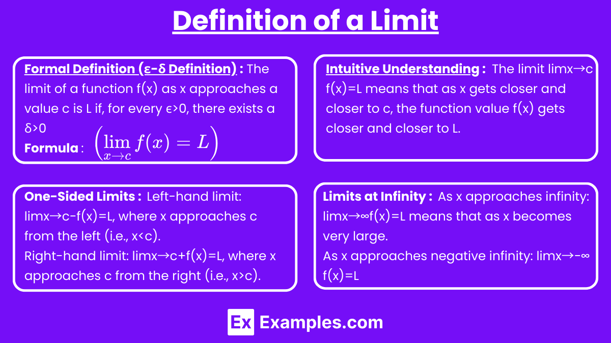
Formal Definition (ε-δ Definition):
The limit of a function f(x) as x approaches a value c is L if, for every ϵ>0, there exists a δ>0 such that whenever 0<∣x−c∣<δ, it follows that ∣f(x)−L∣<ϵ. This is written as:

Intuitive Understanding:
- The limit limx→cf(x)=L means that as x gets closer and closer to c, the function value f(x) gets closer and closer to L.
- The limit does not necessarily mean f(x)=L at x=c, only that f(x) approaches L as x approaches c.
One-Sided Limits:
- Left-hand limit: limx→c−f(x)=L, where x approaches c from the left (i.e., x<c).
- Right-hand limit: limx→c+f(x)=L, where x approaches c from the right (i.e., x>c).
Limits at Infinity:
- As x approaches infinity: limx→∞f(x)=L means that as x becomes very large, f(x) approaches L.
- As x approaches negative infinity: limx→−∞f(x)=L implies that as x becomes very large in the negative direction, f(x) approaches L.
Properties of Limits
Properties of limits include basic rules like the sum, difference, product, and quotient rules, which allow us to calculate the limit of a combination of functions by breaking them down into simpler parts. Additionally, the limit of a constant is the constant itself, and the limit of a function as x approaches a value applies directly to that function, provided it is continuous at that point.
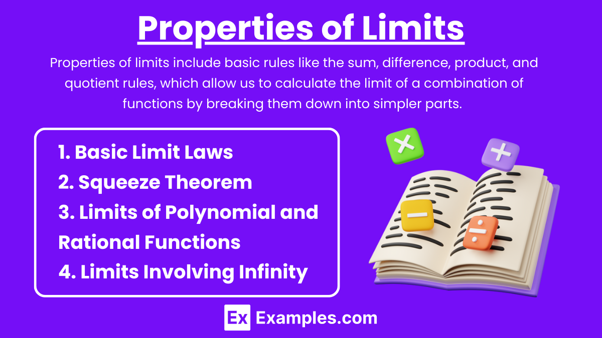
1. Basic Limit Laws
These laws help simplify complex limit calculations by breaking them down into simpler parts.
- Sum Law:
![\left(\lim_{x \to c} [f(x) + g(x)] = \lim_{x \to c} f(x) + \lim_{x \to c} g(x)\right)](https://www.examples.com/wp-content/ql-cache/quicklatex.com-1ae71391aa76b66df028f8375ee82a3c_l3.png "Rendered by QuickLaTeX.com")
- Difference Law:
![\left(\lim_{x \to c} [f(x) - g(x)] = \lim_{x \to c} f(x) - \lim_{x \to c} g(x)\right)](https://www.examples.com/wp-content/ql-cache/quicklatex.com-85ffd8364a99cccf9dcca75170d85233_l3.png "Rendered by QuickLaTeX.com")
- Product Law:
![\left(\lim_{x \to c} [f(x) \cdot g(x)] = \lim_{x \to c} f(x) \cdot \lim_{x \to c} g(x)\right)](https://www.examples.com/wp-content/ql-cache/quicklatex.com-f3c6fc5707c1ce4a90093e63c543b25b_l3.png "Rendered by QuickLaTeX.com")
- Quotient Law:
![\left(\lim_{x \to c} \left[\frac{f(x)}{g(x)}\right] = \frac{\lim_{x \to c} f(x)}{\lim_{x \to c} g(x)}, \text{ provided } \lim_{x \to c} g(x) \neq 0\right)](https://www.examples.com/wp-content/ql-cache/quicklatex.com-43d5603bfe17a221c824a70ece0daeb4_l3.png "Rendered by QuickLaTeX.com")
- Constant Multiple Law:
![\left(\lim_{x \to c} [k \cdot f(x)] = k \cdot \lim_{x \to c} f(x)\right)](https://www.examples.com/wp-content/ql-cache/quicklatex.com-838ce1afbebf042264fb9620924a96b3_l3.png "Rendered by QuickLaTeX.com")
- Power Law:
![\left(\lim_{x \to c} [f(x)]^n = \left[\lim_{x \to c} f(x)\right]^n\right)](https://www.examples.com/wp-content/ql-cache/quicklatex.com-c69ce8998a422c6c1c0724aeab208a27_l3.png "Rendered by QuickLaTeX.com")
2. Squeeze Theorem
If g(x)≤f(x)≤h(x) for all x near c (except possibly at c), and if limx→cg(x)=limx→ch(x)=L, then limx→cf(x)=L.
3. Limits of Polynomial and Rational Functions
- Polynomial Functions:

- where p(x) is any polynomial function.
- Rational Functions:

4. Limits Involving Infinity
- For rational functions, consider the degrees of the numerator and denominator:
- Top-heavy (numerator degree > denominator degree): limx→∞q(x)p(x)=∞ or −∞.
- Bottom-heavy (numerator degree < denominator degree): limx→∞q(x)p(x)=0.
- Equal degree: limx→∞q(x)p(x) equals the ratio of leading coefficients.
Representations of Limits
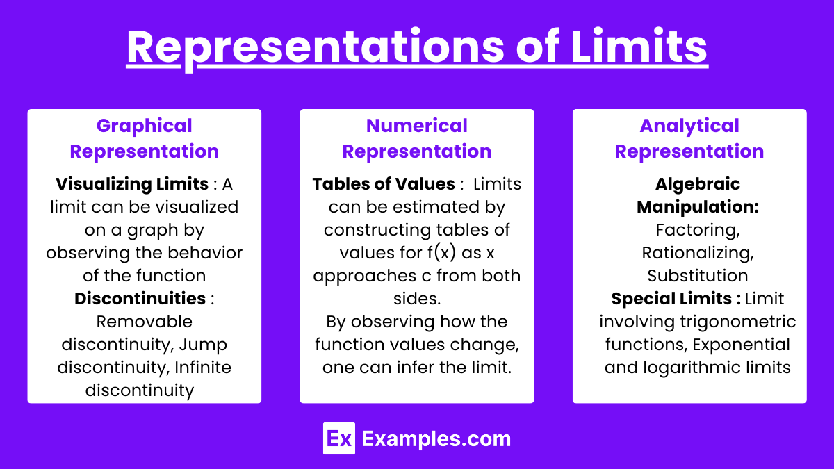
1. Graphical Representation
- Visualizing Limits:
- A limit can be visualized on a graph by observing the behavior of the function as it approaches the point x=c.
- The limit is the y-value the function approaches as x nears c, not necessarily the value the function actually reaches.
- Discontinuities:
- Removable discontinuity: The limit exists, but f(x) is not defined at x=c or differs from the limit.
- Jump discontinuity: The left-hand limit and right-hand limit exist but are not equal.
- Infinite discontinuity: The function approaches infinity or negative infinity as x approaches c.
2. Numerical Representation
- Tables of Values:
- Limits can be estimated by constructing tables of values for f(x) as x approaches c from both sides.
- By observing how the function values change, one can infer the limit.
3. Analytical Representation
- Algebraic Manipulation:
- Factoring: Simplify the expression by factoring to cancel terms that may cause indeterminate forms like 00.
- Rationalizing: Multiply by the conjugate to eliminate square roots.
- Substitution: Directly substitute x=c into the function if no indeterminate form arises.
- Special Limits:
- Limit involving trigonometric functions: x→0limxsinx=1
- Exponential and logarithmic limits: x→0+limln(x)=−∞,x→∞lime−x=0
Examples
Example 1: Limit of a Function at a Point
For the function  , to find the limit as x approaches 1, substitute x=1 directly and you’ll get an indeterminate form. By factoring the numerator to (x−1)(x+1) and canceling out (x−1), the limit simplifies to limx→1f(x)=2.
Example 2: One-Sided Limits
Consider  . The limit as x approaches 2 from the left (x→2−) is −∞ because the function approaches negative infinity as you get closer to 2 from the left side. However, from the right (x→2+), it approaches +∞.
Example 3: Infinite Limits
Take  . As x approaches 0, the function becomes very large in value, moving towards infinity. Thus, limx→0 1/x2 = ∞.
Example 4 : Limits at Infinity
For  , as x approaches infinity, the terms with lower degrees in the numerator and denominator become insignificant. So, the limit becomes limx→∞f(x)=2.
Example 5: Limit with Substitution
If you have f(x)=x3+2x+1, finding the limit as xxx approaches 2 is straightforward. By substituting x=2, you get limx→2f(x)=8+4+1=13. This shows a simple application where limits can be found by direct substitution when the function is continuous at that point.
Multiple Choice Questions
Question 1
Which of the following best describes the limit of a function f(x) as x approaches a value c?
A) The value of f(x) at x=c.
B) The value that f(x) approaches as x gets infinitely close to c.
C) The average of the values of f(x) around x=c.
D) The value that f(x) approaches as x gets infinitely large.
Correct Answer: B
Explanation: The limit of a function f(x) as x approaches a value c is defined as the value that f(x) approaches as x gets infinitely close to c. It does not necessarily mean the value of the function at c, and it is not related to the average value of the function around c. Answer D refers to the concept of limits at infinity, which is a different scenario.
Question 2
Which of the following is true about the limit limx→cf(x) when the left-hand limit and right-hand limit are not equal?
A) The limit exists and is equal to the average of the left-hand and right-hand limits.
B) The limit exists and is equal to the left-hand limit.
C) The limit does not exist.
D) The limit exists and is equal to the right-hand limit.
Correct Answer: C
Explanation: For the limit limx→cf(x) to exist, both the left-hand limit limx→c−f(x) and the right-hand limit limx→c+f(x) must be equal. If they are not equal, the overall limit does not exist. Thus, Answer C is correct.
Question 3
Given limx→2f(x)=5 and limx→2g(x)=3, what is limx→2[f(x)+g(x)]?
A) 15
B) 8
C) 5
D) Does not exist
Correct Answer: B
Explanation: The limit of the sum of two functions is equal to the sum of their individual limits. Given limx→2f(x)=5 and limx→2g(x)=3, we can find limx→2[f(x)+g(x)]=limx→2f(x)+limx→2g(x)=5+3=8. Therefore, the correct answer is B.