Deriving and Applying a Model for Exponential Growth and Decay

In AP Calculus AB and BC, exponential growth and decay models are fundamental for understanding how quantities change over time. These models describe situations where the rate of change of a quantity is proportional to the quantity itself. This concept is essential in fields such as biology, economics, and physics. By deriving the exponential function from a simple differential equation, students can apply it to various real-world scenarios, making it a crucial topic for mastering both AP Calculus exams.

Learning Objectives

When studying “Deriving and Applying a Model for Exponential Growth and Decay” for the AP Calculus AB and BC exams, you should focus on understanding how to derive the exponential growth and decay models from first-order differential equations. Learn to interpret the significance of the growth/decay constant 𝑘, and apply these models to solve real-world problems involving population growth, radioactive decay, and continuously compounded interest. Master solving problems related to half-life, doubling time, and continuous growth/decay scenarios using these models.

Understanding Exponential Growth and Decay

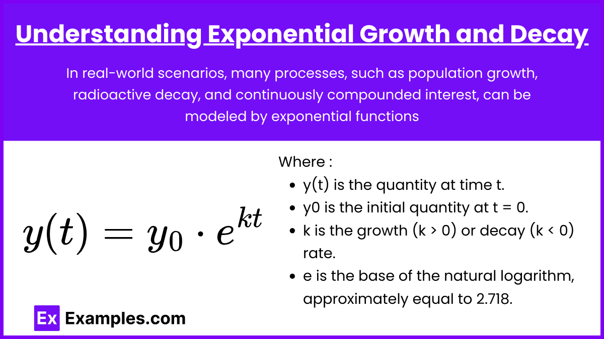
In real-world scenarios, many processes, such as population growth, radioactive decay, and continuously compounded interest, can be modeled by exponential functions.

• Exponential Growth occurs when a quantity increases over time.
• Exponential Decay occurs when a quantity decreases over time.

The general form of an exponential function is:

\(y(t) = y_0 \cdot e^{kt} \)

Where:

• y(t) is the quantity at time t.
• y0​ is the initial quantity at t = 0.
• k is the growth (k > 0) or decay (k < 0) rate.
• e is the base of the natural logarithm, approximately equal to 2.718.

Deriving the Exponential Growth and Decay Model

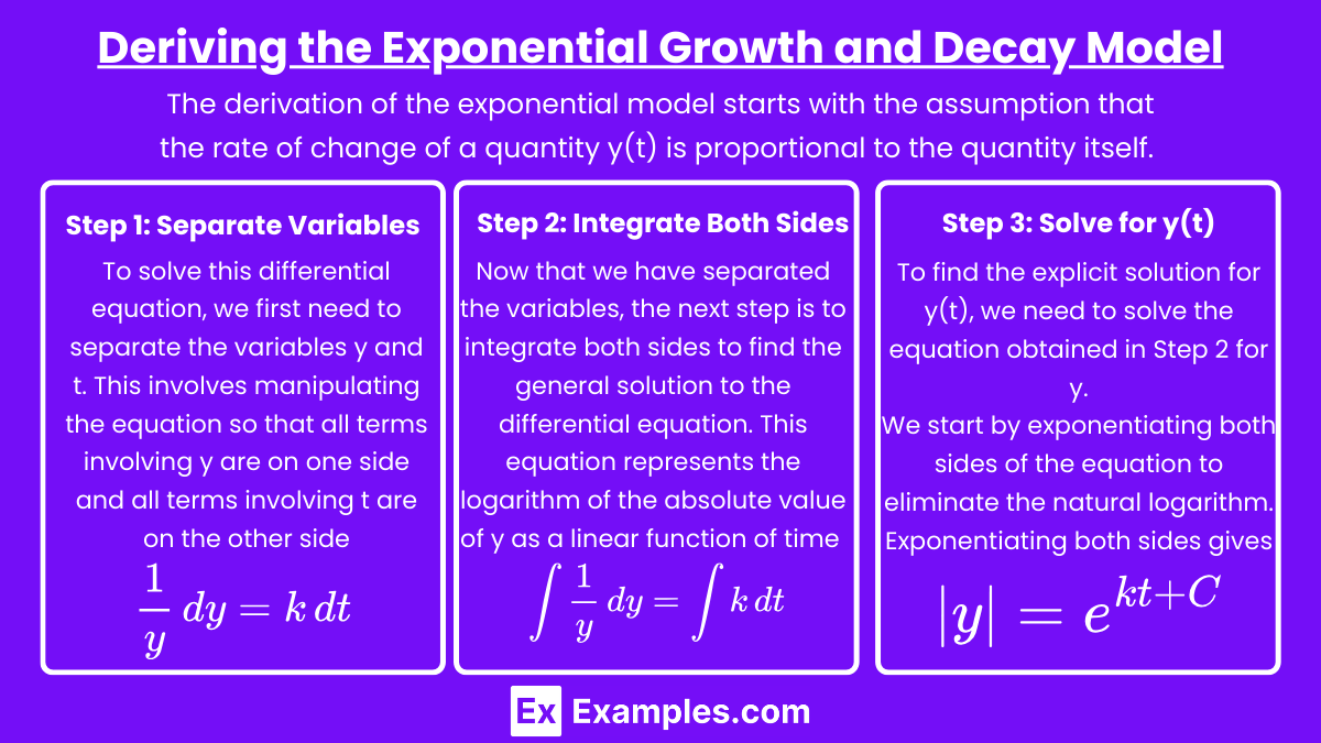
The derivation of the exponential model starts with the assumption that the rate of change of a quantity y(t) is proportional to the quantity itself. Mathematically, this is expressed as :

\(\frac{dy}{dt} = ky(t) \)

This is a first-order differential equation. The solution to this differential equation gives us the model for exponential growth or decay.

Step 1: Separate Variables

• To solve this differential equation, we first need to separate the variables y and t. This involves manipulating the equation so that all terms involving y are on one side and all terms involving t are on the other side:
• This separation allows us to integrate both sides with respect to their respective variables, which leads us to the next step.

\(\frac{1}{y} \, dy = k \, dt \)

Step 2: Integrate Both Sides

• Now that we have separated the variables, the next step is to integrate both sides to find the general solution to the differential equation.

\(\int \frac{1}{y} \, dy = \int k \, dt \)

\(\ln |y| = kt + C \)

This equation represents the logarithm of the absolute value of y as a linear function of time t.

Step 3: Solve for y(t)

• To find the explicit solution for y(t), we need to solve the equation obtained in Step 2 for y.
• We start by exponentiating both sides of the equation to eliminate the natural logarithm. Exponentiating both sides gives

\(|y| = e^{kt+C} \)

Since e^kt+C can be rewritten as e^kt⋅ e^C , and because e^C is itself a constant, we can write:

\(y(t) = Ae^{kt} \)

Apply the initial condition y(0) = y₀​

\(y_0 = Ae^{k \cdot 0} = A \)

Therefore, the solution is

\(y(t) = y_0 e^{kt} \)

This is the exponential growth and decay model.

Applying the Exponential Growth and Decay Model

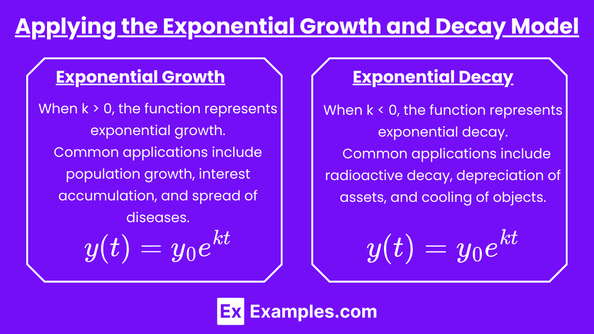
1. Exponential Growth

• When k > 0, the function \( y(t) = y_0 e^{kt} \) represents exponential growth.
• Common applications include population growth, interest accumulation, and spread of diseases.

Example: Suppose a population of 100 bacteria grows at a rate of 5% per hour. The growth model is: \(y(t) = 100 \cdot e^{0.05t} \)

To find the population after 10 hours: \(y(10) = 100 \cdot e^{0.05 \cdot 10} \approx 164.87 \)

2. Exponential Decay

• When k < 0, the function \( y(t) = y_0 e^{kt} \) represents exponential decay.
• Common applications include radioactive decay, depreciation of assets, and cooling of objects.

Example: A radioactive substance decays at a rate of 3% per hour. If the initial amount is 200 grams, the decay model is: \(y(t) = 200 \cdot e^{-0.03t} \)

To find the amount remaining after 5 hours: \(y(5) = 200 \cdot e^{-0.03 \cdot 5} \approx 171.77 \text{ grams} \)

Key Concepts for AP Calculus AB and BC

1. Rate of Change Interpretation

• The differential equation \( \frac{dy}{dt} = ky \) shows that the rate of change is proportional to the quantity. This is crucial for understanding how rapidly quantities grow or decay.

2. Half-Life and Doubling Time

• Half-Life (for decay) is the time it takes for a quantity to reduce to half its initial value. It can be derived using the equation \( t_{1/2} = \frac{\ln 2}{|k|} \)​.
• Doubling Time (for growth) is the time it takes for a quantity to double. It can be derived using \( t_{2x} = \frac{\ln 2}{k} \)​.

Example (Doubling Time): If a population grows at a rate of 7% per year, the doubling time is: \(t_{2x} = \frac{\ln 2}{0.07} \approx 9.9 \text{ years} \)

3. Solving Real-World Problems

• On the AP Calculus exam, you might be given a scenario and asked to set up and solve an exponential model. Be sure to understand how to extract key information like the initial value, growth/decay rate, and time intervals from word problems.

Examples

Example 1: Bacterial Population Growth

Suppose a certain type of bacteria doubles in number every 3 hours. If you start with 500 bacteria, the population can be modeled by the exponential growth function y(t) = 500 ⋅ e^kt. To find the growth rate k, use the fact that the population doubles when t = 3, so 1000 = 500⋅e^3k. Solving this gives \( k = \frac{\ln 2}{3} \approx 0.231 \). Therefore, the population at any time t is y(t) = 500⋅e^0.231t.

Example 2: Radioactive Decay

A radioactive substance has a half-life of 10 years. If the initial amount is 120 grams, the decay of the substance can be modeled by y(t) = 120⋅e^kt. The half-life condition gives 60 = 120⋅e^10k. Solving this, \( k = \frac{\ln 0.5}{10} \approx -0.0693 \). The amount of the substance after t years is then given by y(t) = 120⋅e^−0.0693t.

Example 3: Continuous Compound Interest

An initial investment of $5,000 is placed in an account that earns 4% interest per year, compounded continuously. The amount of money in the account after t years is given by the model A(t) = 5000⋅e^0.04t. To find the balance after 8 years, substitute t = 8 into the equation, yielding A(8) ≈ 5000⋅e^0.32 ≈ 6835.38. This shows that the investment will grow to approximately $6,835.38 after 8 years.

Example 4: Carbon-14 Dating

The amount of Carbon-14 in a fossil decays exponentially over time, with a half-life of 5,730 years. If a fossil originally had 10 grams of Carbon-14 and now has only 2 grams, the time elapsed can be calculated using the decay model y(t) = 10⋅e^kt. Knowing \( k = \frac{\ln 0.5}{5730} \approx -0.00012097 \), we can solve 2 = 10⋅e^{−0.00012097t} to find t ≈ 13344 years. This suggests the fossil is approximately 13,344 years old.

Example 5: Pharmacokinetics

A drug is administered intravenously, and its concentration in the bloodstream decreases exponentially as the body metabolizes it. Suppose the drug has an initial concentration of 200 mg/L and a half-life of 4 hours. The decay of the drug’s concentration over time can be modeled by \( C(t) = 200 \cdot e^{kt} \), where \( k = \frac{\ln 0.5}{4} \approx -0.1733 \). The concentration of the drug after 12 hours is C(12) = 200⋅e^{−0.1733⋅12} ≈ 25 mg/L, indicating that the concentration has dropped significantly over this period.

Multiple Choice Questions

Question 1

The population of a certain species of fish in a lake is modeled by the function P(t) = 200⋅e^0.04t, where P(t) represents the population at time t in years. What is the approximate population after 5 years?

A) 200
B) 244
C) 245
D) 250

Answer: C) 245

Explanation:

To find the population after 5 years, substitute t = 5 into the given exponential model:

P(5) = 200⋅e^0.04×5

Calculate the exponent:

P(5) = 200⋅e^0.2

Using e^0.2 ≈ 1.221, we get:

P(5) ≈ 200⋅1.221 = 244.2

Rounding to the nearest whole number, the population is approximately 245.

Question 2

A substance decays according to the function N(t) = N_0​⋅e^−0.1t, where N(t) is the amount remaining at time t and N₀​ is the initial amount. If N_0​ = 100 grams, how much of the substance remains after 10 hours?

A) 36.8 grams
B) 50 grams
C) 60.6 grams
D) 90.5 grams

Answer: A) 36.8 grams

Explanation:

To find the amount remaining after 10 hours, substitute t = 10 into the exponential decay model:

N(10) = 100⋅e^−0.1 × 10

Simplify the exponent:

N(10) = 100⋅e⁻¹

Using e⁻¹ ≈ 0.368, we get:

N(10) ≈ 100⋅0.368 = 36.8 grams

So, after 10 hours, approximately 36.8 grams of the substance remains.

Question 3

If a population doubles every 5 years, what is the value of the constant k in the exponential growth model P(t) = P₀​⋅e^kt?

A) \( \frac{\ln 2}{5} \)
B) \( \ln 2 \)
C) \( 5 \ln 2 \)
D) \( \frac{1}{5} \)

Answer: A) \( \frac{\ln 2}{5} \)

Explanation:

The doubling time of a population is the time Td​ it takes for the population to double, which satisfies:

\(P(T_d) = 2P_0 = P_0 \cdot e^{kT_d} \)

Dividing both sides by P₀​:

\(2 = e^{kT_d} \)

Taking the natural logarithm of both sides:

\(\ln 2 = kT_d \)

Solving for k:

\(k = \frac{\ln 2}{T_d} \)

Given that the doubling time Td​ is 5 years:

\(k = \frac{\ln 2}{5} \)

Therefore, the value of k is \( \frac{\ln 2}{5} \)​.

These questions and detailed explanations are designed to test and reinforce your understanding of exponential growth and decay, a crucial topic for AP Calculus.