Generalizing Understandings of Motion Problems to other Situations Involving Rates of Change

In AP Calculus, motion problems provide a fundamental framework for understanding rates of change. These problems typically involve analyzing an object’s position, velocity, and acceleration over time. By mastering these concepts, students can generalize this understanding to a wide range of real-world scenarios, such as population growth, economic trends, and fluid dynamics. Recognizing how derivatives and integrals describe the rates of change in various contexts is essential for success in both AP Calculus AB and BC, where such applications are frequently tested.

Learning Objectives

By studying “Generalizing Understandings of Motion Problems to Other Situations Involving Rates of Change” for the AP Calculus AB and BC exams, you should learn to interpret and apply the concepts of derivatives and integrals beyond physical motion, including areas like population growth, fluid flow, and economic models. You should be able to analyze and solve related rates problems, understand the significance of first and second derivatives in various contexts, and generalize the principles of position, velocity, and acceleration to different real-world scenarios.

Key Concepts

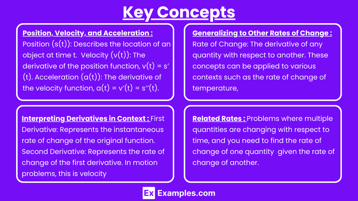
1. Position, Velocity, and Acceleration

Position (s(t)): Describes the location of an object at time t.
Velocity (v(t)): The derivative of the position function, v(t) = s′(t). It represents the rate of change of position with respect to time.
Acceleration (a(t)): The derivative of the velocity function, a(t) = v′(t) = s′′(t). It represents the rate of change of velocity with respect to time.

2. Generalizing to Other Rates of Change

Rate of Change: The derivative of any quantity with respect to another (e.g., dy/dx where y is a function of x).
Contextual Application: These concepts can be applied to various contexts such as the rate of change of temperature, population growth, or the rate of water being pumped into a tank.

3. Interpreting Derivatives in Context

First Derivative: Represents the instantaneous rate of change of the original function. In motion problems, this is velocity; in other contexts, it could be the rate of growth or the speed of an economic indicator.
Second Derivative: Represents the rate of change of the first derivative. In motion problems, this is acceleration; in other contexts, it could be the rate at which the rate of growth is changing (e.g., the acceleration of a population increase).

4. Related Rates

Related Rates: Problems where multiple quantities are changing with respect to time, and you need to find the rate of change of one quantity given the rate of change of another.
Example: If the radius of a balloon is increasing over time, how fast is the volume of the balloon changing?

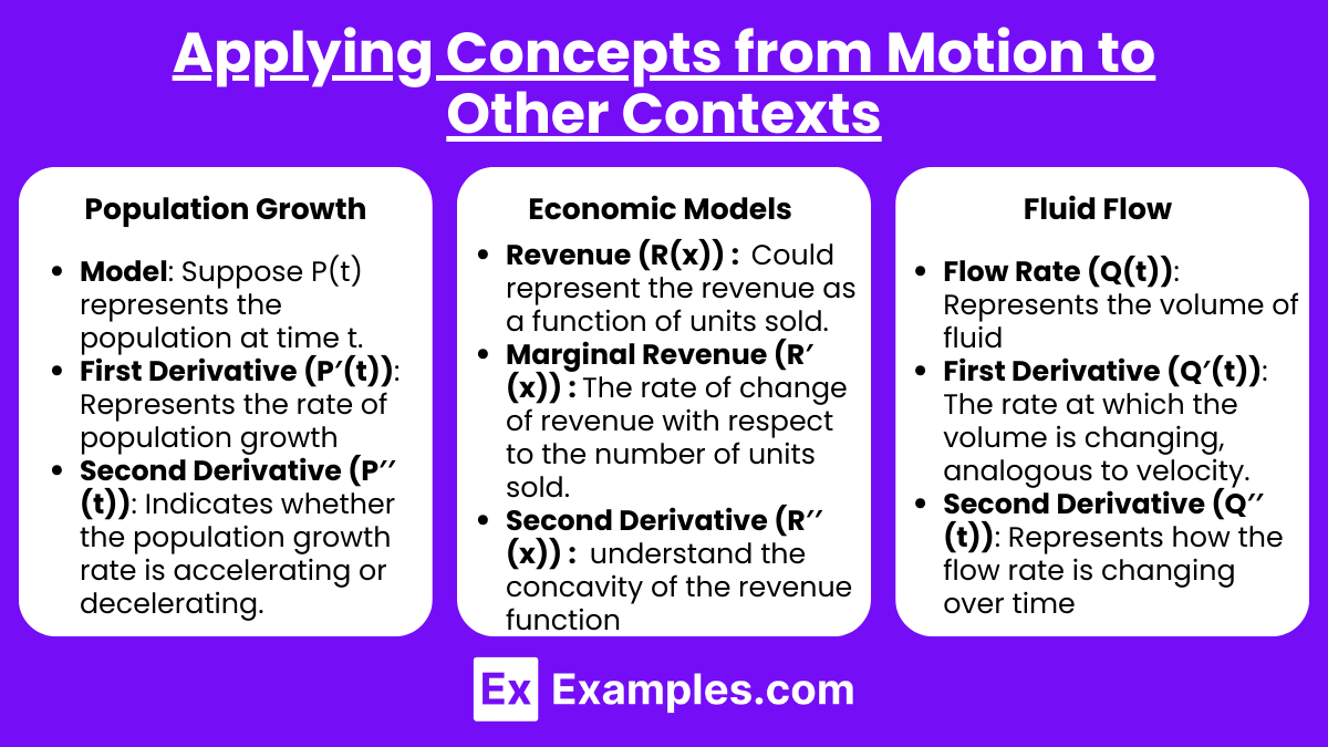
Applying Concepts from Motion to Other Contexts

1. Population Growth

Model: Suppose P(t) represents the population at time t.
First Derivative (P′(t)): Represents the rate of population growth (e.g., people per year).
Second Derivative (P′′(t)): Indicates whether the population growth rate is accelerating or decelerating.

2. Economic Models

Revenue (R(x)): Could represent the revenue as a function of units sold.
Marginal Revenue (R′(x)): The rate of change of revenue with respect to the number of units sold, showing how much revenue increases per additional unit sold.
Second Derivative (R′′(x)): Can help understand the concavity of the revenue function and whether the marginal revenue is increasing or decreasing.

3. Fluid Flow

Flow Rate (Q(t)): Represents the volume of fluid passing through a pipe over time.
First Derivative (Q′(t)): The rate at which the volume is changing, analogous to velocity.
Second Derivative (Q′′(t)): Represents how the flow rate is changing over time, analogous to acceleration.

Strategies for Success on the AP Calculus Exam

1. Understand the Underlying Principles

Don’t just memorize formulas; understand what they mean and how they apply in different contexts.
Be able to explain in words what a derivative or integral represents in the context of the problem.

2. Practice Generalizing

Work on problems from various contexts to practice applying your understanding of derivatives and integrals to new situations.
For example, practice transitioning from motion problems to problems involving the rate of change of temperature or the spread of a disease.

3. Solve Related Rates Problems

These problems are common in both AP Calculus AB and BC. Practice identifying the relationship between different quantities and their rates of change.
Draw diagrams, if possible, to visualize the relationships between the variables.

4. Use Multiple Representations

Be comfortable with graphical, numerical, and analytical representations of functions.
Understand how to interpret the meaning of derivatives and integrals in graphs, and how these can inform the behavior of the function in real-world scenarios.

5. Work Through Free Response Questions

The AP Calculus exams often include free-response questions that require you to interpret, generalize, and apply your understanding to new situations.
Practice with past exam questions to get used to the format and types of questions asked.

Examples

Example 1: Population Growth Analysis

Just as velocity represents the rate of change of position over time, population growth can be modeled with a function where the first derivative represents the rate of growth. For instance, if a city’s population is modeled by a function P(t), then P′(t) shows how quickly the population is increasing or decreasing at any given time. The second derivative P′′(t) indicates whether the growth rate itself is accelerating or decelerating.

Example 2: Economic Marginal Analysis

In economics, the concept of marginal revenue can be understood similarly to velocity in motion problems. If R(x) represents the revenue function based on the number of units sold, then the first derivative R′(x) gives the marginal revenue, indicating the rate at which revenue changes with each additional unit sold. The second derivative R′′(x) helps analyze whether the marginal revenue is increasing or decreasing, much like acceleration in motion.

Example 3: Thermal Dynamics

Consider the rate of change of temperature in a cooling object. If T(t) represents the temperature at time t, the first derivative T′(t) would represent how quickly the temperature is dropping or rising over time, analogous to velocity. The second derivative T′′(t) could indicate whether the rate of cooling is speeding up or slowing down, similar to acceleration in motion problems.

Example 4: Fluid Dynamics

The rate at which water flows into or out of a tank can be modeled similarly to motion along a line. If V(t) represents the volume of water in the tank at time t, then the first derivative V′(t) would represent the rate of flow (e.g., gallons per minute). The second derivative V′′(t) would indicate whether the rate of flow is increasing or decreasing, similar to acceleration in a motion context.

Example 5: Spread of Disease

In epidemiology, the spread of an infectious disease can be modeled by a function I(t) representing the number of infected individuals over time. The first derivative I′(t) would then indicate the rate at which the disease is spreading (e.g., new cases per day), much like velocity. The second derivative I′′(t) would reveal whether the spread is accelerating or decelerating, similar to how acceleration works in motion problems.

Multiple Choice Questions

Question 1

A company’s revenue R(x) from selling x units of a product is given by the function R(x) = 100x − 0.5x². What does the first derivative R′(x) represent in this context?

a) The total revenue from selling x units
b) The maximum revenue the company can achieve
c) The rate at which revenue changes with respect to the number of units sold
d) The rate at which the number of units sold changes with respect to revenue

Answer: c) The rate at which revenue changes with respect to the number of units sold

Explanation: The first derivative R′(x) of the revenue function R(x) represents the marginal revenue, which is the rate of change of revenue with respect to the number of units sold. It tells you how much the revenue will increase or decrease if you sell one more unit. This concept is analogous to velocity in motion problems, where the first derivative of position gives the rate of change of position with respect to time.

Question 2

The population P(t) of a city is modeled by the function P(t) = 2000e^0.03t, where t is the number of years since 2000. What does the second derivative P′′(t) indicate?

a) The initial population of the city in the year 2000
b) The rate of population growth at time t
c) The acceleration of the population growth at time t
d) The total population in the year 2000

Answer: c) The acceleration of the population growth at time t

Explanation: The second derivative P′′(t) represents the rate of change of the rate of population growth, also known as the acceleration of population growth. Just as in motion problems where the second derivative of position (acceleration) indicates how the velocity is changing, here P′′(t) indicates whether the population is growing faster or slower over time.

Question 3

Water is being pumped into a tank at a rate modeled by the function Q(t) = 4t²+ 3t +2, where Q(t) is the volume of water in gallons at time t in minutes. What is the physical interpretation of the derivative Q′(t)?

a) The total volume of water in the tank at time t
b) The rate at which the volume of water is changing with respect to time
c) The total amount of water that will be pumped into the tank after t minutes
d) The amount of water initially in the tank

Answer: b) The rate at which the volume of water is changing with respect to time

Explanation: The derivative Q′(t) represents the rate of change of the volume of water in the tank with respect to time, which in this context is the flow rate of water being pumped into the tank. This is similar to the concept of velocity in motion problems, where the derivative of the position function gives the rate at which the position changes over time.