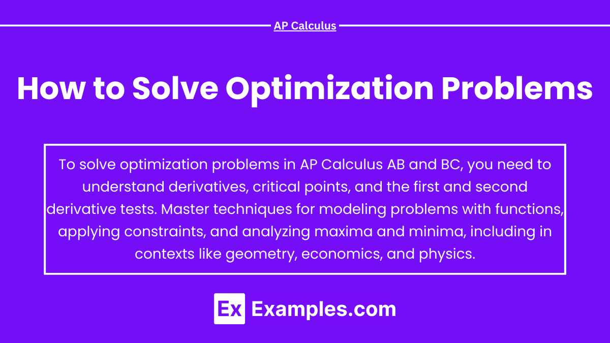
How to Solve Optimization Problems

In AP Calculus AB and BC, optimization problems are a fundamental concept where students learn to find the maximum or minimum values of a function within a given domain. These problems often involve real-world applications, such as maximizing area, minimizing cost, or optimizing resources. By modeling the problem with equations, taking derivatives, and analyzing critical points, students can efficiently solve these problems. Mastering optimization techniques is crucial for success in both AP Calculus AB and BC, as they frequently appear on the exam.

Learning Objectives

By studying optimization problems for the AP Calculus AB and BC exams, you should learn how to model real-world situations using functions, identify and formulate objective functions and constraints, and apply calculus techniques to find and classify critical points. You’ll master using the first and second derivative tests to determine local maxima and minima, and interpret these results within the problem’s context. Additionally, you should be able to solve optimization problems involving parametric equations and polar coordinates, particularly in AP Calculus BC.

Optimization problems are a key topic in AP Calculus AB and BC. These problems involve finding the maximum or minimum values of a function within a given domain, often with real-world applications. Below is a step-by-step guide on how to approach and solve optimization problems, tailored to help you excel in both AP Calculus AB and BC.

What Are Optimization Problems?

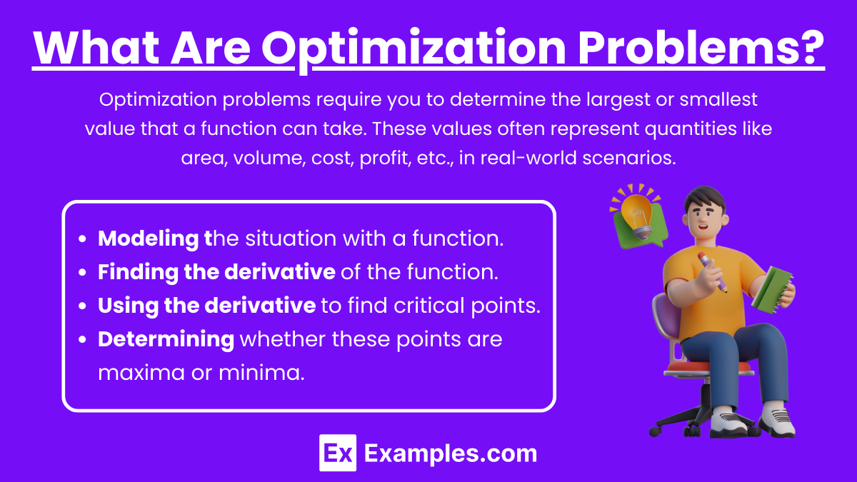
Optimization problems require you to determine the largest or smallest value that a function can take. These values often represent quantities like area, volume, cost, profit, etc., in real-world scenarios. In AP Calculus, solving these problems involves:

Modeling the situation with a function.
Finding the derivative of the function.
Using the derivative to find critical points.
Determining whether these points are maxima or minima.

Step-by-Step Process to Solve Optimization Problems

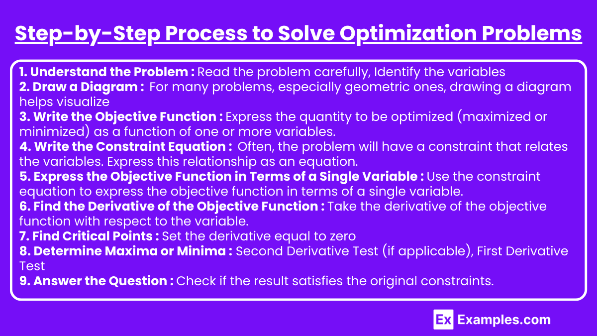
1. Understand the Problem

Read the problem carefully: Identify what quantity needs to be maximized or minimized.
Identify the variables: Assign variables to the quantities involved.

2. Draw a Diagram (if applicable) : Visual representation: For many problems, especially geometric ones, drawing a diagram helps visualize relationships between variables.

3. Write the Objective Function

Objective Function: Express the quantity to be optimized (maximized or minimized) as a function of one or more variables. This is called the objective function.
Example: If you’re asked to minimize the surface area S of a box with a fixed volume V, S would be your objective function.

4. Write the Constraint Equation

Constraints: Often, the problem will have a constraint that relates the variables. Express this relationship as an equation.
Example: For the box, the volume constraint V = l×w×h, where l, w, and h are the length, width, and height, respectively.

5. Express the Objective Function in Terms of a Single Variable

Substitution: Use the constraint equation to express the objective function in terms of a single variable.
Example: If you have S = 2lw+2lh+2wh and the constraint V = lwh, solve the constraint for one variable and substitute it into the surface area formula.

6. Find the Derivative of the Objective Function

Differentiate: Take the derivative of the objective function with respect to the variable.
This derivative, called the first derivative, helps find critical points where the maximum or minimum might occur.

7. Find Critical Points

Set the derivative equal to zero: Solve f′(x) = 0 to find the critical points.
These points are potential candidates for maxima or minima.

8. Determine Maxima or Minima

Second Derivative Test (if applicable): Take the second derivative f′′(x).
- If f′′(x) > 0, the function has a local minimum at that point.
- If f′′(x) < 0, the function has a local maximum at that point.
First Derivative Test: Alternatively, use the first derivative test by analyzing the sign changes of f′(x) around the critical points.

9. Answer the Question

Substitute back: Plug the critical points into the original function to find the maximum or minimum value, and interpret the result in the context of the problem.
Verify: Check if the result satisfies the original constraints.

Optimization Tips for AP Calculus AB and BC

Understand the context: Knowing how to translate a word problem into a mathematical model is crucial.
Practice: Work on various types of optimization problems, including those involving geometry, economics, and physics.
Show all steps: AP exams require clear, logical steps to receive full credit. Even if the final answer is wrong, correctly showing your process can earn you partial credit.
Be thorough: Ensure your critical points are within the domain of the problem and satisfy the constraint equation.

Examples

Example 1. Maximizing Rectangle Area with Fixed Perimeter

You have 40 meters of fencing to create a rectangular garden. To maximize the area, let the length be l and width be w with l+w = 20. The area A is A = l(20−l). Maximize it by setting A′(l) = 20−2l = 0, so l = 10. The garden should be a 10m x 10m square, giving a maximum area of 100 square meters.

Example 2. Minimizing Perimeter of Rectangle with Fixed Area

Minimize the perimeter of a rectangle with an area of 36 square meters. Let l and w be the length and width with l×w = 36. Perimeter $ P = 2l + 2w = 2l + \frac{72}{l} $. Minimize by solving $ P'(l) = 2 – \frac{72}{l^2} = 0 $, so l = 6. The rectangle should be a 6m x 6m square, giving a minimum perimeter of 24 meters.

Example 3. Maximizing Triangle Area with Fixed Hypotenuse

Maximize the area of a right triangle with a fixed hypotenuse of 10 meters. If the legs are x and y, $ A = \frac{1}{2}xy $ with x²+y² = 100. Express $ y = \sqrt{100 – x^2} $ and maximize $ A(x) = \frac{1}{2}x\sqrt{100 – x^2} $. The maximum area is 25 square meters when $ x = y = 5\sqrt{2} $.

Example 4. Minimizing Surface Area of Cylinder with Fixed Volume

Minimize the surface area of a cylinder with a fixed volume of 100 cubic centimeters. With radius r and height $ h = \frac{100}{\pi r^2} $, surface area $ S = 2\pi r^2 + \frac{200}{r} $. Minimize by solving $ S'(r) = 4\pi r – \frac{200}{r^2} = 0 $, leading to $ r = \sqrt[3]{\frac{50}{\pi}} $. This gives the minimal surface area.

Example 5. Maximizing Profit by Setting Optimal Price

Maximize the profit from selling a product at price p per unit, with revenue $ R(p) = 100p – p^2 $. Differentiate to find R′(p) = 100−2p, set it to zero, so p = 50. The optimal price is $50, which maximizes revenue and, consequently, profit at $2500.

Multiple Choice Questions

Question 1

You have 60 meters of fencing to enclose a rectangular garden against an existing wall, so only three sides need fencing. What dimensions of the garden will maximize the area?

A) 20 × 20 meters
B) 15 × 30 meters
C) 30 × 15 meters
D) 10 × 30 meters

Correct Answer: C) 30 × 15 meters

Explanation: Let the width of the garden (perpendicular to the wall) be w and the length (parallel to the wall) be l. The total amount of fencing is given by 2w+l = 60. The area A to be maximized is A = w×l.

Express l in terms of w: l = 60−2w.
Substitute into the area formula: A(w) = w(60−2w)=60w−2w².
Differentiate A(w) to find A′(w) = 60−4w, and set it equal to zero: 60−4w = 0, so w = 15.
Substituting w = 15 back into l = 60−2w, we get l = 30.

Thus, the dimensions 30×15 meters will maximize the area.

Question 2

A company can sell x units of a product at a price p given by p = 200−2x. What quantity x maximizes the revenue?

A) x = 25
B) x = 50
C) x = 75
D) x = 100

Correct Answer: B) x = 50

Explanation: Revenue R(x) is the product of price p and quantity x. Given p = 200−2x, the revenue function is R(x) = x × (200−2x) = 200x−2x².

To maximize revenue, differentiate R(x) with respect to x: R′(x) = 200−4x.
Set R′(x) = 0 to find the critical point: 200−4x = 0, so x = 50.

The quantity x = 50 maximizes revenue.