Local Linearity and Approximation

Local linearity is a critical concept in both AP Calculus AB and BC, describing how a function behaves like a straight line when examined closely around a specific point. This idea is foundational for understanding differentiable functions, tangent lines, and linear approximation. In the AP Calculus exams, students apply local linearity to approximate function values, analyze the behavior of functions near a given point, and connect these ideas to more advanced topics such as Taylor series in Calculus BC. Mastery of this concept is essential for success.

Learning Objectives

For the AP Calculus AB and BC exams, you should focus on understanding the concept of local linearity, including how to determine whether a function is locally linear at a point by analyzing its differentiability. Master the linear approximation method using the tangent line and be able to apply it to estimate function values near a given point. Additionally, in AP Calculus BC, extend your knowledge to include applications of local linearity in differential equations and Taylor series for more advanced problem-solving.

Introduction to Local Linearity

Local linearity is a fundamental concept in calculus that describes how a function behaves like a straight line when you zoom in close enough at a point on its curve. This idea is crucial in understanding the behavior of differentiable functions and serves as the foundation for concepts like linear approximation and tangent lines.

Key Concept: Differentiability and Local Linearity

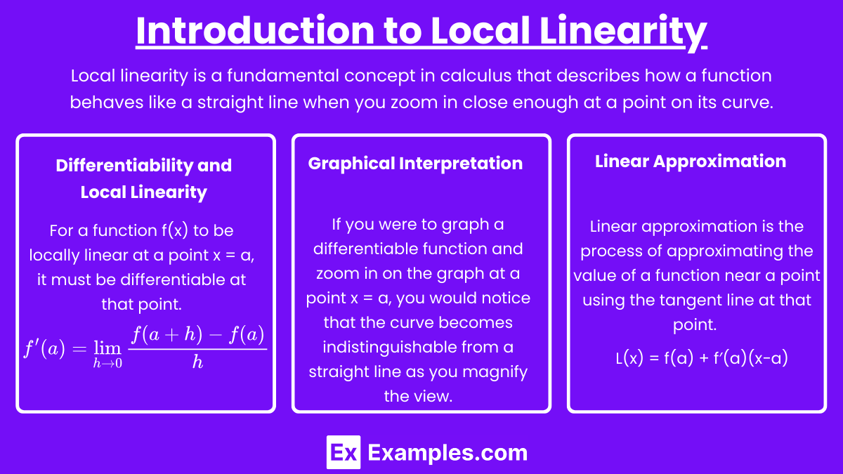
For a function f(x) to be locally linear at a point x = a, it must be differentiable at that point. Differentiability implies that the function’s graph has a well-defined tangent line at x = a, and as you zoom in closer and closer to x = a, the curve of the function increasingly resembles this tangent line. Mathematically, this is captured by the derivative of the function at x = a:

\( f'(a) = \lim_{h \to 0} \frac{f(a+h) – f(a)}{h} \)

This derivative f′(a) represents the slope of the tangent line to the curve at x = a.

Graphical Interpretation

If you were to graph a differentiable function and zoom in on the graph at a point x = a, you would notice that the curve becomes indistinguishable from a straight line as you magnify the view. This straight line is the tangent line at x = a, and the slope of this line is f′(a).

Linear Approximation (Tangent Line Approximation)

Linear approximation is the process of approximating the value of a function near a point using the tangent line at that point. This method is particularly useful when dealing with functions that are difficult to compute directly.

Formula for Linear Approximation

Given a function f(x) that is differentiable at x = a, the linear approximation of f(x) near x = a is given by the equation of the tangent line:

L(x) = f(a) + f′(a)(x−a)

Where:

• L(x) is the linear approximation of f(x) at x near a.
• f(a) is the value of the function at x = a.
• f′(a) is the slope of the tangent line at x = a.

Example

Consider the function \( f(x) = \sqrt{x} \)​ and let’s find the linear approximation near x = 4.

1. Compute f(4): \( f(4) = \sqrt{4} = 2 \)
2. Find the derivative f′(x): \(f'(x) = \frac{1}{2\sqrt{x}}\)
3. Evaluate the derivative at x = 4: \(f'(4) = \frac{1}{2\sqrt{4}} = \frac{1}{4}\)
4. Write the linear approximation formula: \(L(x) = 2 + \frac{1}{4}(x – 4)\)

Thus, the linear approximation of \( f(x) = \sqrt{x} \)​ near x = 4 is:

\(L(x) = 2 + \frac{1}{4}(x – 4)\)

Application: Estimating Values

Using the linear approximation, you can estimate the value of f(x) near x = 4. For instance, to estimate \( \sqrt{4.1} \)

\(L(4.1) = 2 + \frac{1}{4}(4.1 – 4) = 2 + \frac{0.1}{4} = 2 + 0.025 = 2.025\)

Thus, \( \sqrt{4.1} \approx 2.025 \)

Local Linearity in AP Calculus AB and BC

AP Calculus AB

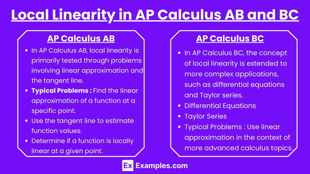
In AP Calculus AB, local linearity is primarily tested through problems involving linear approximation and the tangent line. Students are expected to understand how to derive the tangent line at a given point and use it to approximate function values.

• Typical Problems:
  • Find the linear approximation of a function at a specific point.
  • Use the tangent line to estimate function values.
  • Determine if a function is locally linear at a given point by analyzing its differentiability.

AP Calculus BC

In AP Calculus BC, the concept of local linearity is extended to more complex applications, such as differential equations and Taylor series.

• Differential Equations:
  • Students might use local linearity to approximate solutions to differential equations near an initial condition.
• Taylor Series:
  • The first-degree Taylor polynomial is essentially the linear approximation, and BC students must understand how this connects to local linearity.
• Typical Problems:
  • Use linear approximation in the context of more advanced calculus topics.
  • Analyze the accuracy of linear approximation using Taylor series.

Examples

Example 1: Square Root Function Approximation

Consider the function \( f(x) = \sqrt{x} \)​ near x = 9. The tangent line at x = 9 is used to approximate the value of \( \sqrt{x} \)for values close to 9. For instance, to estimate \( \sqrt{9.1} \)​, you would use the linear approximation \( L(x) = 3 + \frac{1}{6}(x – 9) \), resulting in \( L(9.1) \approx 3.0167 \).

Example 2: Natural Logarithm Approximation

For the function \( f(x) = \ln(x) \) near x = 1, the linear approximation can be found using the tangent line. The derivative f′(1) = 1, so the linear approximation L(x) = x−1 can be used to estimate values like ln(1.1). Thus, ln(1.1)≈0.1.

Example 3: Exponential Function Approximation

The function f(x) = e^x is often approximated near x = 0 using its tangent line. Since f(0) = 1 and f′(0) = 1, the linear approximation is L(x) = 1+x. This can approximate e^0.1 ≈ 1.1.

Example 4: Cosine Function Approximation

The function f(x) = cos(x) near x = 0 can be approximated using the tangent line. With f(0)=1 and f′(0)=0, the linear approximation L(x) = 1 suggests that for small values of x, cos(x) ≈ 1. This approximation works well for values like cos(0.01) ≈ 1.

Example 5: Cubic Function Approximation

For a cubic function such as f(x) = x³ near x = 1, the tangent line provides a linear approximation. Given f(1) = 1 and f′(1) = 3, the linear approximation is L(x) = 1+3(x−1). This approximation can estimate values like 1.1³ ≈ 1.3.

Multiple Choice Questions

Question 1

Which of the following statements is true about the concept of local linearity?

A) A function is locally linear at a point if it has a horizontal tangent line at that point.
B) A function is locally linear at a point if it is differentiable at that point.
C) A function is locally linear at a point only if the derivative at that point is zero.
D) A function is locally linear at a point only if it is continuous at that point.

Answer: B) A function is locally linear at a point if it is differentiable at that point.

Explanation: Local linearity means that when you zoom in sufficiently close to a point on a differentiable function, the graph of the function will look like a straight line, which is the tangent line at that point. Differentiability at a point ensures that the function has a well-defined tangent line, which is a key aspect of local linearity.

Question 2

What is the linear approximation of the function f(x) = x² near x = 2?

A) L(x) = 4+(x−2)
B) L(x) = 4+4(x−2)
C) L(x) = 2x
D) L(x) = 2x−2

Answer: B) L(x) = 4+4(x−2)

Explanation: The linear approximation formula is L(x) = f(a)+f′(a)(x−a). For f(x) = x² at x = 2, f(2) = 4 and f′(x) = 2x, so f′(2) = 4. Substituting into the linear approximation formula, we get L(x) = 4+4(x−2).

Question 3

Using the linear approximation \( L(x) = 3 + \frac{1}{2}(x – 4) \), what is the estimated value of f(4.2)?

A) 3.0
B) 3.1
C) 3.2
D) 3.3

Answer: B) 3.1

Explanation: To find the estimated value of f(4.2) using the linear approximation \( L(x) = 3 + \frac{1}{2}(x – 4) \), substitute x = 4.2 into the formula:

L(4.2) = 3+1/2 ​(4.2−4) = 3+1/2 ​(0.2) = 3+0.1 = 3.1

Thus, the estimated value of f(4.2) is 3.1.