
Modeling Particle Motion

 . It represents the rate of change of the position with respect to time. Velocity indicates the speed and direction of the particle’s movement.
 . It represents the rate of change of velocity with respect to time. Acceleration indicates how quickly the particle is speeding up or slowing down.


 . This scenario illustrates how to model particle motion when the particle experiences constant acceleration.
 . The particle’s acceleration can also be found by differentiating the velocity vector. This example shows how to model the motion of a particle moving along a curved path in the plane.

 . First, we find the first derivative to get the velocity:

Modeling particle motion in AP Calculus AB and BC involves analyzing how a particle moves along a line or in a plane using calculus concepts like derivatives and integrals. Students study the relationships between position, velocity, and acceleration to describe and predict the particle's motion. This topic is crucial for understanding real-world applications of calculus, as it requires interpreting graphs, solving differential equations, and applying the Fundamental Theorem of Calculus to analyze motion in various contexts.
Free AP Calculus AB Practice Test
Free AP Calculus BC Practice Test
Learning Objectives
In learning Modeling Particle Motion for the AP Calculus AB and BC exams, you should focus on understanding how to analyze the position, velocity, and acceleration of a particle moving along a straight line or in a plane. This includes interpreting and sketching graphs, calculating displacement and total distance traveled, and solving problems involving derivatives and integrals of motion functions. Additionally, for AP Calculus BC, you should be proficient with parametric equations, vector-valued functions, and polar coordinates to model more complex motions.
Modeling Particle Motion
Modeling particle motion is a significant topic in both AP Calculus AB and AP Calculus BC. This topic involves understanding how the position, velocity, and acceleration of a particle moving along a straight line change over time. You will use derivatives and integrals to analyze the motion, which can include interpreting graphs, solving differential equations, and applying the Fundamental Theorem of Calculus.
Key Concepts
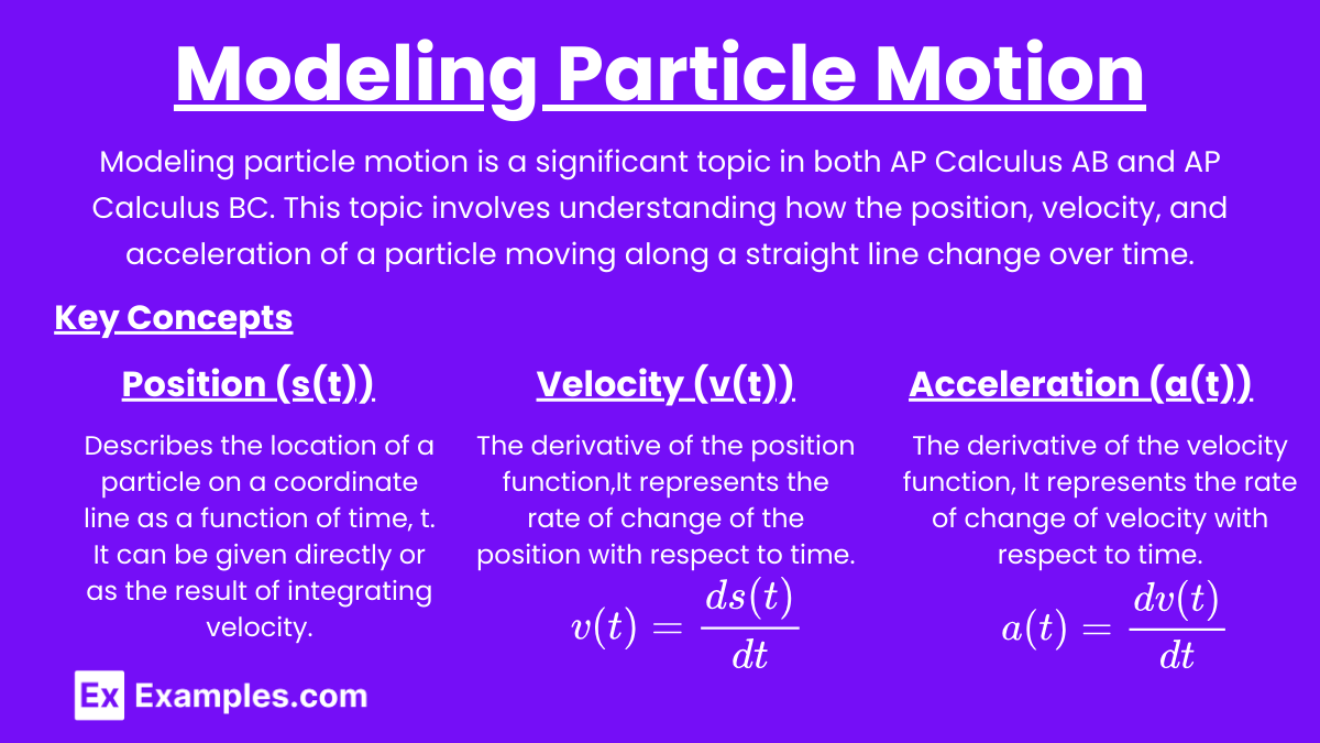
1. Position, Velocity, and Acceleration
Position (s(t)): Describes the location of a particle on a coordinate line as a function of time, t. It can be given directly or as the result of integrating velocity.
Velocity (v(t)): The derivative of the position function, . It represents the rate of change of the position with respect to time. Velocity indicates the speed and direction of the particle's movement.
Acceleration (a(t)): The derivative of the velocity function, . It represents the rate of change of velocity with respect to time. Acceleration indicates how quickly the particle is speeding up or slowing down.
2. Displacement vs. Total Distance Traveled
Displacement: The change in position of the particle over a time interval [t1,t2]. It is calculated as s(t2)−s(t1). Displacement considers direction and can be positive, negative, or zero.
Total Distance Traveled: The total length of the path the particle travels, regardless of direction. It is calculated by integrating the absolute value of the velocity function:
3. Speed
Speed: The absolute value of the velocity function, ∣v(t)∣. Speed is a scalar quantity, meaning it does not consider direction.
4. Interpreting Velocity and Acceleration
When Velocity is Positive (v(t) > 0): The particle is moving to the right or upward.
When Velocity is Negative (v(t) < 0): The particle is moving to the left or downward.
When Velocity is Zero (v(t) = 0): The particle is at rest.
When Acceleration is Positive (a(t) > 0): The velocity is increasing.
When Acceleration is Negative (a(t) < 0): The velocity is decreasing.
When Velocity and Acceleration have the Same Sign: The particle is speeding up.
When Velocity and Acceleration have Opposite Signs: The particle is slowing down.
Integrating Velocity and Acceleration to Find Position and Velocity Functions
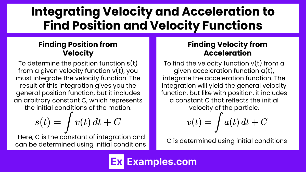
1. Finding Position from Velocity
To determine the position function s(t) from a given velocity function v(t), you must integrate the velocity function. The result of this integration gives you the general position function, but it includes an arbitrary constant C, which represents the initial conditions of the motion. This constant is crucial because it accounts for the specific starting position of the particle.
To find the position function s(t) when given a velocity function v(t), integrate the velocity function:
Here, C is the constant of integration and can be determined using initial conditions (e.g., the initial position s(t0)).
2. Finding Velocity from Acceleration
To find the velocity function v(t) from a given acceleration function a(t), integrate the acceleration function. The integration will yield the general velocity function, but like with position, it includes a constant C that reflects the initial velocity of the particle. To find the velocity function v(t) when given an acceleration function a(t), integrate the acceleration function:
Again, C is determined using initial conditions (e.g., the initial velocity v(t0)).
Graphical Analysis
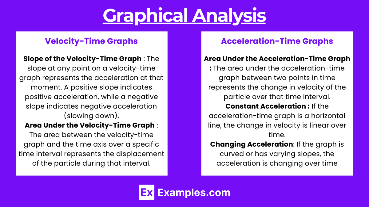
Velocity-Time Graphs
Slope of the Velocity-Time Graph: The slope at any point on a velocity-time graph represents the acceleration at that moment. A positive slope indicates positive acceleration (speeding up), while a negative slope indicates negative acceleration (slowing down). A zero slope (a horizontal line) indicates constant velocity.
Area Under the Velocity-Time Graph: The area between the velocity-time graph and the time axis over a specific time interval represents the displacement of the particle during that interval. If the graph lies above the time axis, the displacement is positive, indicating motion in the positive direction. If the graph is below the time axis, the displacement is negative, indicating motion in the opposite direction. The total area, considering the sign, gives the net displacement.
Acceleration-Time Graphs
Area Under the Acceleration-Time Graph: The area under the acceleration-time graph between two points in time represents the change in velocity of the particle over that time interval. A positive area (above the time axis) indicates an increase in velocity, while a negative area (below the time axis) indicates a decrease in velocity.
Constant Acceleration: If the acceleration-time graph is a horizontal line (constant acceleration), the change in velocity is linear over time.
Changing Acceleration: If the graph is curved or has varying slopes, the acceleration is changing over time, which results in a non-linear change in velocity.
Advanced Topics for AP Calculus BC
1. Parametric Equations
In AP Calculus BC, particles may move in a plane rather than along a line. This motion is described using parametric equations x(t) and y(t).
Velocity in Parametric Form:
Acceleration in Parametric Form:
2. Vector-Valued Functions
Another extension in AP Calculus BC is modeling particle motion using vector-valued functions.
Position Vector:
Velocity Vector:
Acceleration Vector:
3. Polar Coordinates (BC Only)
Position in Polar Form: r(θ)
Velocity and Acceleration: Derived from the derivatives of r(θ) and the angle θ(t).
Examples
Example 1: Particle with Given Velocity Function
Suppose a particle moves along a straight line with a velocity function v(t) = 4t−2 where t represents time in seconds. To find the particle's position at any time t, you would integrate the velocity function to obtain the position function s(t). If the initial position s(0) is given as 3 meters, the position function becomes s(t) = 2t2−2t+3. This example demonstrates how to determine the position of a particle given its velocity function.
Example 2: Particle Moving Under Constant Acceleration
Consider a particle initially at rest that begins moving with a constant acceleration of a(t) = 5 m/s2. Since the particle starts from rest, the initial velocity v(0) = 0. Integrating the acceleration function, we obtain the velocity v(t)=5t. Further integration gives the position function . This scenario illustrates how to model particle motion when the particle experiences constant acceleration.
Example 3: Harmonic Motion
A particle oscillates back and forth along a straight line according to the position function s(t) = 3cos(2t), where t is time in seconds. The velocity and acceleration of the particle can be found by differentiating the position function. Specifically, the velocity function is v(t) = −6sin(2t), and the acceleration function is a(t) = −12cos(2t). This example models the motion of a particle undergoing harmonic motion, such as a mass attached to a spring.
Example 4: Projectile Motion
A particle is projected vertically upward from the ground with an initial velocity of 20 m/s under the influence of gravity (acceleration a(t) = −9.8 m/s2). The velocity function is v(t) = 20−9.8t, and integrating this gives the position function s(t) = 20t−4.9t2. By setting s(t) = 0, you can find the time when the particle returns to the ground. This example illustrates modeling the vertical motion of a projectile under gravity.
Example 5: Particle Moving Along a Plane Curve
Consider a particle moving along a curve in the plane, described by the parametric equations x(t) = t2 and y(t) = t3−3t. The velocity vector of the particle is v(t) = (2t)i+(3t2−3)j, and the speed at any time t is given by . The particle’s acceleration can also be found by differentiating the velocity vector. This example shows how to model the motion of a particle moving along a curved path in the plane.
Multiple Choice Questions
Question 1
A particle moves along a straight line with a velocity function given by v(t) = t2−4t+3, where t is in seconds. At what time(s) is the particle at rest?
A) t = 1 and t = 3
B) t = 0 and t = 4
C) t = 1 and t = 3
D) t = 0.5 and t = 2.5
Answer: C) t = 1 and t = 3
Explanation:
A particle is at rest when its velocity is zero, i.e., v(t) = 0. Setting the given velocity function equal to zero, we solve: t2−4t+3 = 0
This quadratic equation can be factored as: (t−1) (t−3) = 0
Thus, the solutions are t = 1 and t = 3. Therefore, the particle is at rest at these times.
Question 2
Given the position function of a particle s(t) = t3−6t2+9t+2, what is the velocity of the particle at t = 2?
A) 3
B) 0
C) −3
D) 4
Answer: B) 0
Explanation:
The velocity of the particle is the derivative of the position function, . First, we find the derivative of the position function:
Now, substitute t=2 into the velocity function:
Therefore, the correct answer is 0.
Question 3
A particle's position is given by s(t) = 2t2−3t+1. What is the acceleration of the particle?
A) 4t−3
B) 4
C) 2
D) 4t
Answer: B) 4
Explanation:
The acceleration of the particle is the second derivative of the position function, . First, we find the first derivative to get the velocity:
Next, we find the second derivative to obtain the acceleration:
Since the second derivative is a constant, the acceleration of the particle is 4. Therefore, the correct answer is 4.