Sketching Slope Fields and Families of Solution Curves

In AP Calculus AB and BC, understanding slope fields and families of solution curves is essential for mastering differential equations. Slope fields provide a visual representation of a differential equation by showing the slope of the solution curve at various points in the plane. By sketching these fields, students can better understand how solutions behave without solving the equation explicitly. This concept is crucial for interpreting and solving first-order differential equations, making it a key topic for success in both AP Calculus exams.

Free AP Calculus AB Practice Test

Free AP Calculus BC Practice Test

Learning Objectives

When studying “Sketching Slope Fields and Families of Solution Curves” for the AP Calculus AB and BC exams, you should focus on several key objectives. These include learning to accurately sketch slope fields for a given differential equation, interpreting the direction and behavior of solution curves, and identifying how different initial conditions affect the family of solutions. Additionally, you should understand how to approximate solutions using slope fields and connect these concepts to real-world scenarios, such as modeling population growth or motion.

Sketching Slope Fields and Families of Solution Curves

In both AP Calculus AB and AP Calculus BC, the topic of slope fields and families of solution curves is crucial for understanding differential equations. These concepts are commonly tested and understanding them thoroughly can help you achieve a higher score on the exam.

What are Slope Fields?

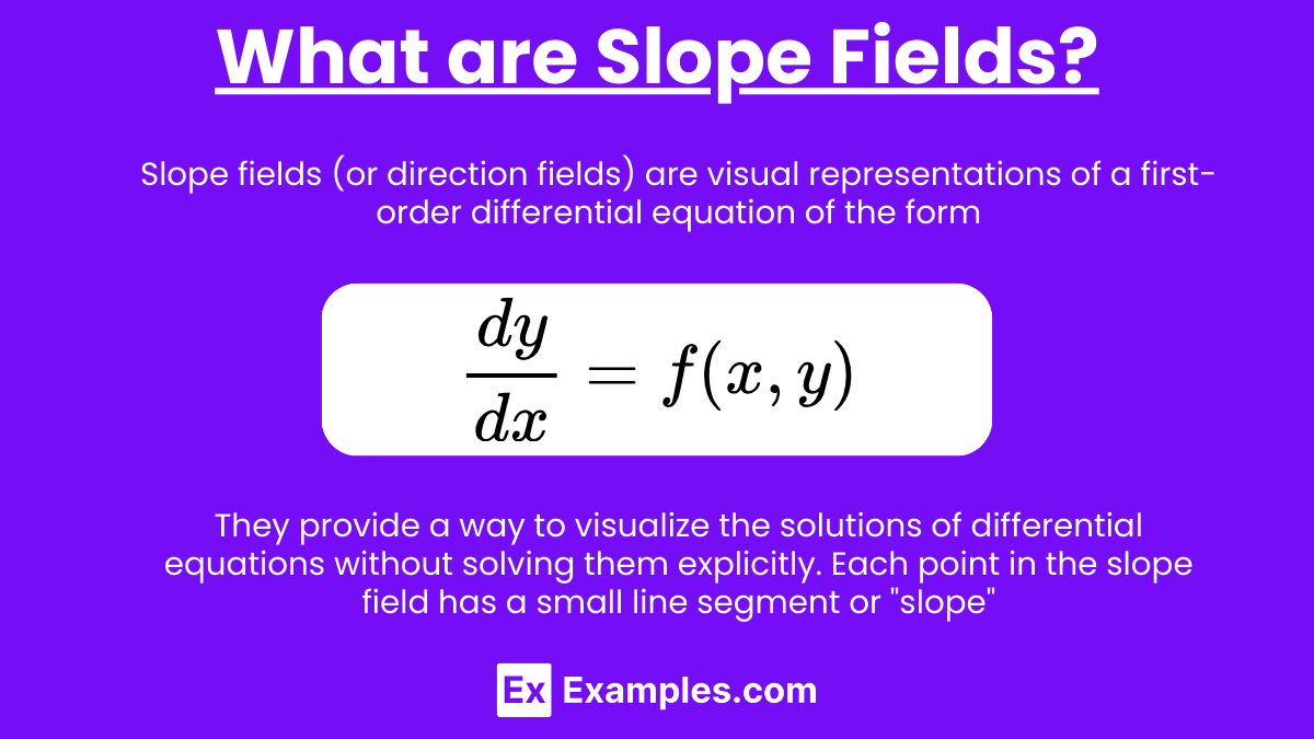
Slope fields (or direction fields) are visual representations of a first-order differential equation of the form:

\(\frac{dy}{dx} = f(x, y) \)

They provide a way to visualize the solutions of differential equations without solving them explicitly. Each point in the slope field has a small line segment or “slope” that represents the value of \(\frac{dy}{dx}\) at that particular (x,y) coordinate.

Steps to Sketch a Slope Field

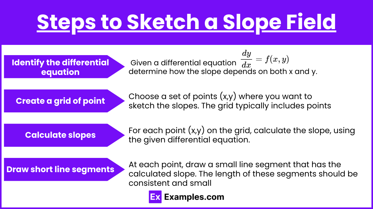
Identify the differential equation: Given a differential equation \(\frac{dy}{dx} = f(x, y)\), determine how the slope depends on both x and y.
Create a grid of points: Choose a set of points (x,y) where you want to sketch the slopes. The grid typically includes points that cover a reasonable range of values for x and y.
Calculate slopes: For each point (x,y) on the grid, calculate the slope \(\frac{dy}{dx}\) using the given differential equation.
Draw short line segments: At each point, draw a small line segment that has the calculated slope. The length of these segments should be consistent and small, as they only indicate direction, not magnitude.

Example of Sketching a Slope Field

Consider the differential equation \(\frac{dy}{dx} = x – y\).

At the point (0,0), the slope is \(\frac{dy}{dx} = 0 – 0 = 0\), so draw a horizontal line segment.
At (1,0), the slope is \(\frac{dy}{dx} = 1 – 0 = 1\), so draw a line segment with a slope of 1.
At (0,1), the slope is \(\frac{dy}{dx} = 0 – 1 = -1\), so draw a line segment with a slope of -1.

Repeat this process for several points to complete the slope field.

Understanding Families of Solution Curves

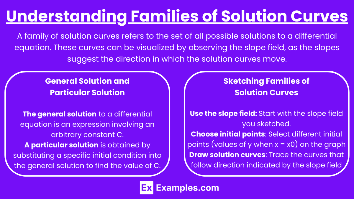
A family of solution curves refers to the set of all possible solutions to a differential equation. These curves can be visualized by observing the slope field, as the slopes suggest the direction in which the solution curves move.

General Solution and Particular Solution

General Solution: The general solution to a differential equation is an expression involving an arbitrary constant C. For example, the general solution to \(\frac{dy}{dx} = k\) (a simple differential equation) is \(y = kx + C\).
Particular Solution: A particular solution is obtained by substituting a specific initial condition into the general solution to find the value of C.

Sketching Families of Solution Curves

Use the slope field: Start with the slope field you sketched. The direction of the slopes will guide the shape of the solution curves.
Choose initial points: Select different initial points (values of y when x = x₀) on the graph. These points correspond to different particular solutions.
Draw solution curves: Trace the curves that follow the direction indicated by the slope field, ensuring they smoothly pass through the initial points.

Example with Initial Conditions

For the differential equation \(\frac{dy}{dx} = x – y\), the general solution is \(y = x – 1 + Ce^{-x}\), where C is an arbitrary constant.

If the initial condition is y(0) = 1, then the particular solution is \(y = x – 1 + 2e^{-x}\).
If the initial condition is y(0) = 0, then the particular solution is \(y = x – 1 + e^{-x}\).

These curves will differ based on the initial conditions but all will follow the direction suggested by the slope field.

Tips for Success

Practice sketching: Be comfortable with quickly sketching slope fields and recognizing the patterns in solution curves.
Understand key differential equations: Common types like \(\frac{dy}{dx} = ky\) (exponential growth/decay) or \(\frac{dy}{dx} = x^2 – y^2\) should be second nature.
Relate to real-world scenarios: Many problems are modeled by differential equations in physics, biology, and economics. Understanding the context can help you interpret the slope fields and solution curves better.
Work on approximation: Use the slope fields to approximate values of the solution at specific points, especially when dealing with initial value problems.

Examples

Example 1: Linear Differential Equation

Consider the differential equation \( \frac{dy}{dx} = 2x \). The slope field for this equation consists of lines with slopes determined by 2x at each point (x,y). As you move along the x-axis, the slope increases linearly. When sketching, you’ll notice that the slope lines become steeper as x increases. The family of solution curves is parabolic and can be expressed as y = x²+C, where C is a constant.

Example 2: Exponential Growth

For the differential equation \( \frac{dy}{dx} = y \), the slope at each point is proportional to the value of y. The slope field will show lines that become steeper as you move away from the x-axis, indicating exponential growth. The family of solution curves is \( y = Ce^x \), representing exponential functions that either grow or decay depending on the value of C.

Example 3: Logistic Growth

Consider the logistic differential equation \( \frac{dy}{dx} = y(1 – y) \). The slope field for this equation shows lines that indicate rapid growth when y is small, slowing as y approaches 1. This creates a curve where the solution curves level off, forming an S-shape. The family of solutions tends to the carrying capacity, described by \( y = \frac{1}{1 + Ce^{-x}} \).

Example 4: Harmonic Oscillator

For the differential equation \( \frac{d^2y}{dx^2} + y = 0 \), sketching the slope field involves recognizing that it represents simple harmonic motion. The slope field displays cyclic patterns, where the slopes indicate the sinusoidal behavior of the solutions. The family of solution curves is \( y = A\cos(x) + B\sin(x) \), depicting the oscillatory motion typical of harmonic oscillators.

Example 5: Autonomous Differential Equation

Consider the equation \( \frac{dy}{dx} = y(2 – y) \). The slope field for this equation shows equilibrium points at y = 0 and y = 2, where the slopes are zero. Solution curves that start between 0 and 2 tend to stabilize at y = 2, while those below zero approach zero. The family of solution curves illustrates how solutions either grow towards the stable equilibrium or decay towards zero, depending on the initial condition.

Multiple Choice Questions

Question 1

Which of the following best describes a slope field for the differential equation \( \frac{dy}{dx} = x \)?

A) The slope at each point depends only on the value of y.
B) The slope at each point depends only on the value of x.
C) The slope at each point is constant across the entire field.
D) The slope at each point depends on both x and y.

Correct Answer: B

Explanation: The differential equation \( \frac{dy}{dx} = x \) indicates that the slope at each point in the slope field depends solely on the value of x. For any fixed value of x, the slope will be constant along the horizontal line at that x-value, regardless of the value of y. Therefore, the correct answer is B. Option A is incorrect because the slope depends only on x, not y. Option C is incorrect because the slope changes with x. Option D is incorrect because the slope does not depend on y.

Question 2

Given the slope field of \( \frac{dy}{dx} = y \), which of the following represents the general family of solution curves?

A) y = x+C
B) y = e^x+C
C) y = Ce^x
D) y = Cx²

Correct Answer: C

Explanation: The differential equation \( \frac{dy}{dx} = y \) has a general solution of the form y = Ce^x, where C is an arbitrary constant. This form of the solution arises because the rate of change of y is proportional to y itself, leading to an exponential growth or decay. Option A represents a linear function, which does not match the behavior described by the differential equation. Option B represents an exponential function with an additional constant term, but it does not represent the general solution to this equation. Option D represents a quadratic function, which also does not match the exponential behavior of the solution.

Question 3

For the differential equation \( \frac{dy}{dx} = y(2 – y) \), what is the behavior of the solution curves as y approaches the equilibrium points?

A) Solution curves will always move away from both equilibrium points.
B) Solution curves will always move towards both equilibrium points.
C) Solution curves will move towards y = 2 and away from y = 0.
D) Solution curves will move away from y = 2 and towards y = 0.

Correct Answer: C

Explanation: The differential equation \( \frac{dy}{dx} = y(2 – y) \) has two equilibrium points at y = 0 and y = 2. By analyzing the behavior near these points, we find that y = 0 is an unstable equilibrium (solution curves move away from it), and y = 2 is a stable equilibrium (solution curves move towards it). Therefore, solution curves tend to approach y = 2 over time, making it a stable point, while they move away from y = 0, indicating that it is unstable. Hence, the correct answer is C.