Searching and Sorting Using Standard Algorithms

In AP Computer Science A, understanding searching and sorting algorithms is fundamental for efficiently managing and processing data. Searching algorithms like linear search and binary search help locate specific values in arrays, while sorting algorithms such as selection sort, insertion sort, merge sort, and quicksort organize data systematically. These algorithms vary in efficiency, with time complexities from O(n) to O(n log n), making it essential to choose the appropriate one based on the data set’s size and structure for optimal performance.

Learning Objectives

For the topic “Searching and Sorting Using Standard Algorithms” in AP Computer Science A, you should aim to understand how to implement, analyze, and select appropriate searching algorithms (like linear and binary search) and sorting algorithms (such as selection, insertion, merge, and quick sort). Focus on grasping the time and space complexities of each algorithm, the conditions in which each is most efficient, and how they operate on different data sets. Master the implementation in Java and understand their applications in real-world problem-solving, specifically within the AP Computer Science A framework.

Searching Algorithms

Linear Search

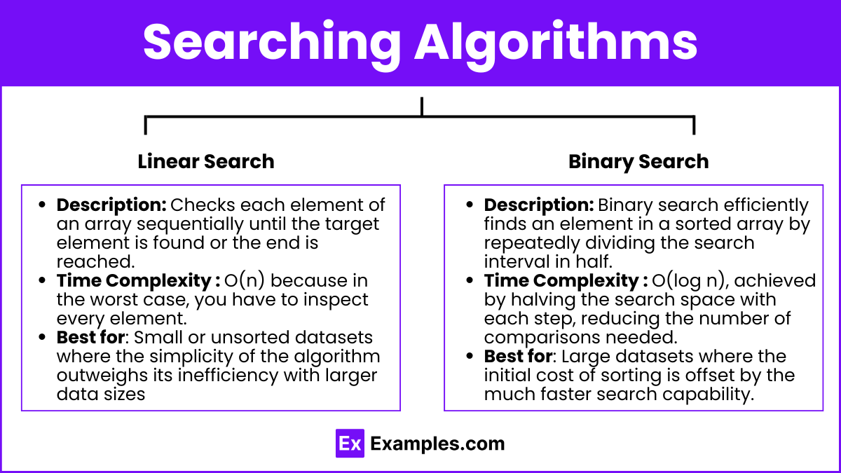
• Description: Linear search checks each element of an array sequentially until the target element is found or the end of the array is reached. It’s a straightforward method that does not require any sorting of the elements beforehand. Checks each element of an array sequentially until the target element is found or the end is reached.
• Time Complexity: O(n) because in the worst case, you have to inspect every element.
• Best for: Small or unsorted data sets. Small or unsorted datasets where the simplicity of the algorithm outweighs its inefficiency with larger data sizes. Also, it’s useful when the data frequently changes, negating the advantage of a sorted structure needed for more efficient searches.

Binary Search

• Description: Binary search efficiently finds an element in a sorted array by repeatedly dividing the search interval in half. It compares the middle element of the array to the target value and discards the half that does not contain the target, continuing the search in the remaining half.
• Time Complexity: O(log n), achieved by halving the search space with each step, significantly reducing the number of comparisons needed.
• Requirements: Array must be sorted prior to the search.
• Best for: Large datasets. Large datasets where the initial cost of sorting is offset by the much faster search capability. It’s especially effective in scenarios where multiple searches are performed on the same data, maximizing the sorting effort.

Sorting Algorithms

1. Selection Sort:
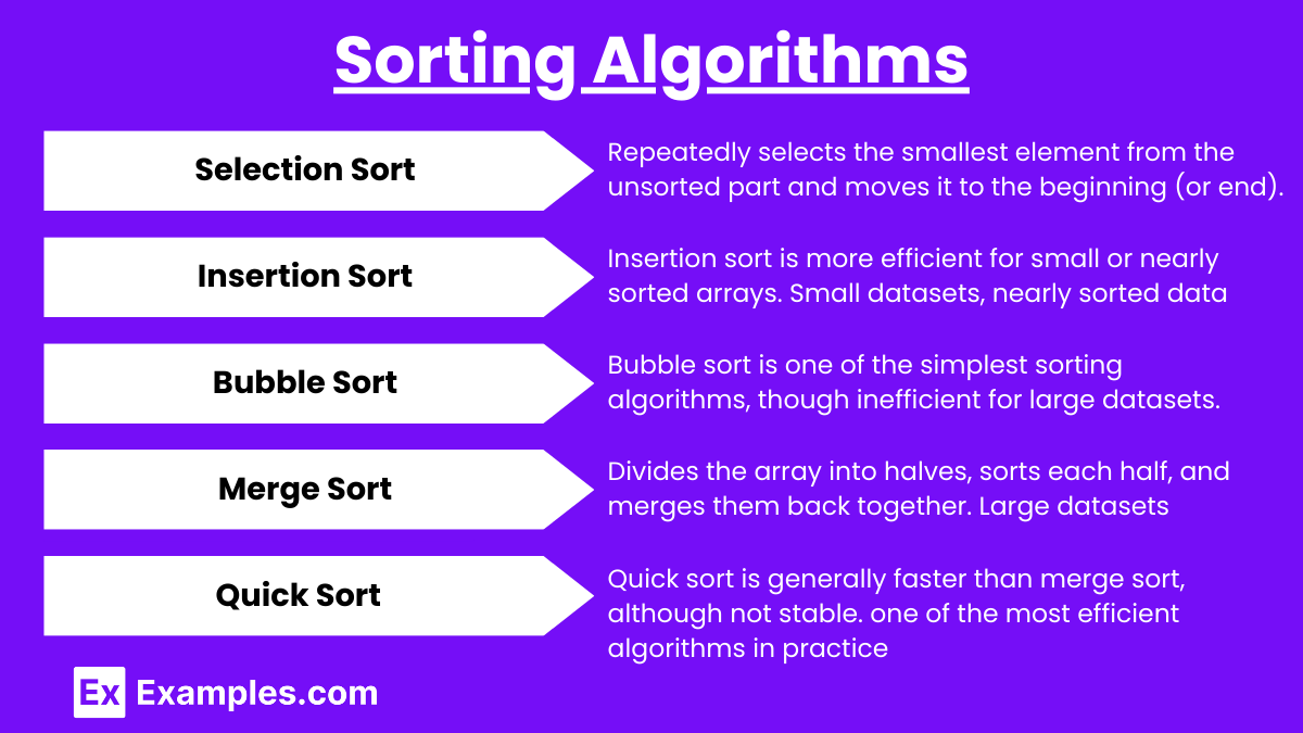
   • Description: Repeatedly selects the smallest (or largest) element from the unsorted part and moves it to the beginning (or end). Selection sort works by dividing the array into a sorted and an unsorted part.
   • Time Complexity: O(n^2) because of nested loops; each pass selects the next smallest element.
   • Best for: Simplicity, small datasets, or when memory is a constraint, but it is inefficient for large arrays.
2. Insertion Sort:
   • Description: Insertion sort is more efficient for small or nearly sorted arrays. It builds a sorted array by repeatedly picking the next element from the unsorted portion and inserting it into the correct position in the sorted portion.
   • Time Complexity: O(n^2) in the worst case; more efficient if the array is nearly sorted.
   • Best for: Small datasets, nearly sorted data, or when you need a simple and adaptive algorithm.
3. Bubble Sort:
   • Description: Bubble sort is one of the simplest sorting algorithms, though inefficient for large datasets. It works by repeatedly stepping through the array, comparing adjacent elements, and swapping them if they are in the wrong order. Repeatedly steps through the list, compares adjacent elements, and swaps them if they are in the wrong order.
   • Time Complexity: O(n^2) in the worst and average cases.
   • Best for: Educational purposes or very small datasets. Bubble sort is mainly used as a teaching tool due to its simple implementation and clear mechanics.
4. Merge Sort:
   • Description: Divides the array into halves, sorts each half, and merges them back together. Merge sort is a recursive divide-and-conquer algorithm that divides the array into halves, recursively sorts each half, and then merges them back together.
   • Time Complexity: O(n log n) consistently, which makes it efficient for larger datasets.
   • Best for: Large datasets where stability (maintaining relative order of equal elements) is important. Merge sort is also well-suited for linked lists because of its non-in-place nature.
5. Quick Sort:
   • Description: Quick sort is one of the most efficient algorithms in practice. It selects a pivot element from the array, partitions the elements into two groups (those smaller than the pivot and those larger), and then recursively sorts the partitions.
   • Time Complexity: O(n log n) on average; O(n^2) in the worst case.
   • Best for: Large datasets due to its high efficiency in practice. Quick sort is generally faster than merge sort, although not stable.

When to Use Each Algorithm

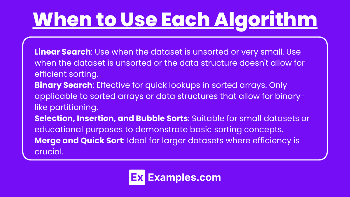
• Linear Search: Use when the dataset is unsorted or very small. Use when the dataset is unsorted or the data structure doesn’t allow for efficient sorting. Works for any type of array, including arrays with duplicates or unsorted collections.
• Binary Search: Effective for quick lookups in sorted arrays. Only applicable to sorted arrays or data structures that allow for binary-like partitioning. Ideal for situations where the dataset is too large to be traversed linearly.
• Selection, Insertion, and Bubble Sorts: Suitable for small datasets or educational purposes to demonstrate basic sorting concepts. These algorithms are typically easy to implement and understand, which makes them good for small applications where efficiency isn’t critical.
• Merge and Quick Sort: Ideal for larger datasets where efficiency is crucial.
  • Merge Sort:Often used in external sorting (e.g., sorting data stored on disk) because of its divide-and-conquer approach and predictable time complexity.
  • Quick Sort: Performs well in most situations, especially for large in-memory datasets. It’s often the default choice for general-purpose sorting algorithms.

Examples

Example 1: Linear Search to Find a Student’s Name in a Roster

Imagine you have an unsorted list of student names and need to find a specific student. A linear search would iterate through each name one by one, checking for a match with the target name. This method is straightforward and works well for small or unsorted lists, but it can be inefficient for larger data sets as it requires checking every element.

Example 2 : Binary Search for Locating a Word in a Dictionary

A binary search is highly efficient when working with sorted data, such as a dictionary. If you are looking for a specific word, binary search will start in the middle of the sorted list, comparing the target word to the middle word. Based on the comparison, it either searches the left or right half of the list, continuously halving the search space until the word is found or the list is exhausted.

Example 3: Selection Sort to Organize Books by Height on a Shelf

Selection sort can be applied to a task such as sorting books by height on a shelf. You would repeatedly select the shortest book from the unsorted portion of the shelf and place it at the beginning. This process continues, selecting the next shortest book, until the entire shelf is sorted by height. Although simple, this approach is inefficient for large collections of books.

Example 4: Insertion Sort for Sorting Playing Cards in Hand

In a card game, you might use insertion sort to arrange cards in your hand by suit or number. As each new card is dealt, you insert it into its proper position among the already sorted cards. This algorithm works well for small numbers of cards or when the hand is almost sorted, making it a practical real-world example of the insertion sort algorithm.

Example 5: Merge Sort for Organizing Large Customer Databases

In a company database with a large number of customer records, merge sort can efficiently sort customer data, such as names or account numbers. The algorithm splits the database into smaller segments, sorts them, and then merges them back together. This divide-and-conquer approach allows for highly efficient sorting of vast amounts of data, making it suitable for large databases.

Multiple Choice Questions

Question 1:

Which of the following is true about binary search?

A) Binary search can be applied to any unsorted array.
B) Binary search has a worst-case time complexity of O(n).
C) Binary search is more efficient than linear search for sorted arrays.
D) Binary search requires additional memory for sorting the array first.

Answer: C

Explanation: Binary search is designed for sorted arrays and works by repeatedly dividing the search interval in half. It is much more efficient than linear search for sorted arrays because its time complexity is O(log n), while linear search’s time complexity is O(n). The array must be sorted first (which isn’t handled by binary search itself), so option D is incorrect. Option A is false because binary search only works on sorted arrays, and option B is incorrect since the worst-case complexity of binary search is O(log n), not O(n).

Question 2:

Which sorting algorithm has the best average-case time complexity for large datasets?

A) Selection Sort
B) Insertion Sort
C) Quick Sort
D) Bubble Sort

Answer: C

Explanation: Quick Sort has an average-case time complexity of O(n log n), making it one of the most efficient algorithms for large datasets. While its worst-case complexity is O(n^2), careful pivot selection can help avoid this. Selection Sort, Insertion Sort, and Bubble Sort all have average and worst-case time complexities of O(n^2), making them less efficient for large datasets compared to Quick Sort.

Question 3:

What is the main drawback of the Merge Sort algorithm compared to Quick Sort?

A) Merge Sort has a worse time complexity.
B) Merge Sort is more difficult to implement.
C) Merge Sort requires additional memory space.
D) Merge Sort cannot be applied to large datasets.

Answer: C

Explanation: The main drawback of Merge Sort is that it requires additional memory space, specifically O(n) auxiliary space, for merging the divided arrays. Although it has a time complexity of O(n log n), which is optimal, the space requirement can be a disadvantage in memory-constrained environments. Option A is incorrect because Merge Sort and Quick Sort both have average-case time complexities of O(n log n). Merge Sort is not necessarily harder to implement than Quick Sort (option B), and it can be applied to large datasets (option D).