The Production Function

Last Updated: October 3, 2024

Notes

In AP Microeconomics, the production function is a fundamental concept that illustrates the relationship between inputs and the resulting output in the production process. It demonstrates how firms utilize various factors of production, such as labor and capital, to generate goods and services efficiently. By analyzing the production function, students gain insights into productivity, cost management, and the principles of increasing and diminishing returns. Understanding this relationship is essential for comprehending how businesses optimize resources to achieve maximum output and maintain competitive advantage.

Free AP Microeconomics Practice Test

Learning Objectives

When studying “The Production Function” for AP Microeconomics, you should aim to understand how different inputs—such as labor and capital—combine to produce output. Grasp the distinctions between short-run and long-run production, including the law of variable proportions and returns to scale. Learn to calculate and interpret total, marginal, and average products, and analyze how technological changes shift the production function. Additionally, master the use of isoquants and isocosts to determine cost-efficient input combinations. These objectives will enable you to apply production theory effectively in various economic scenarios and exam questions.

The Production Function

1. Introduction of The Production Function

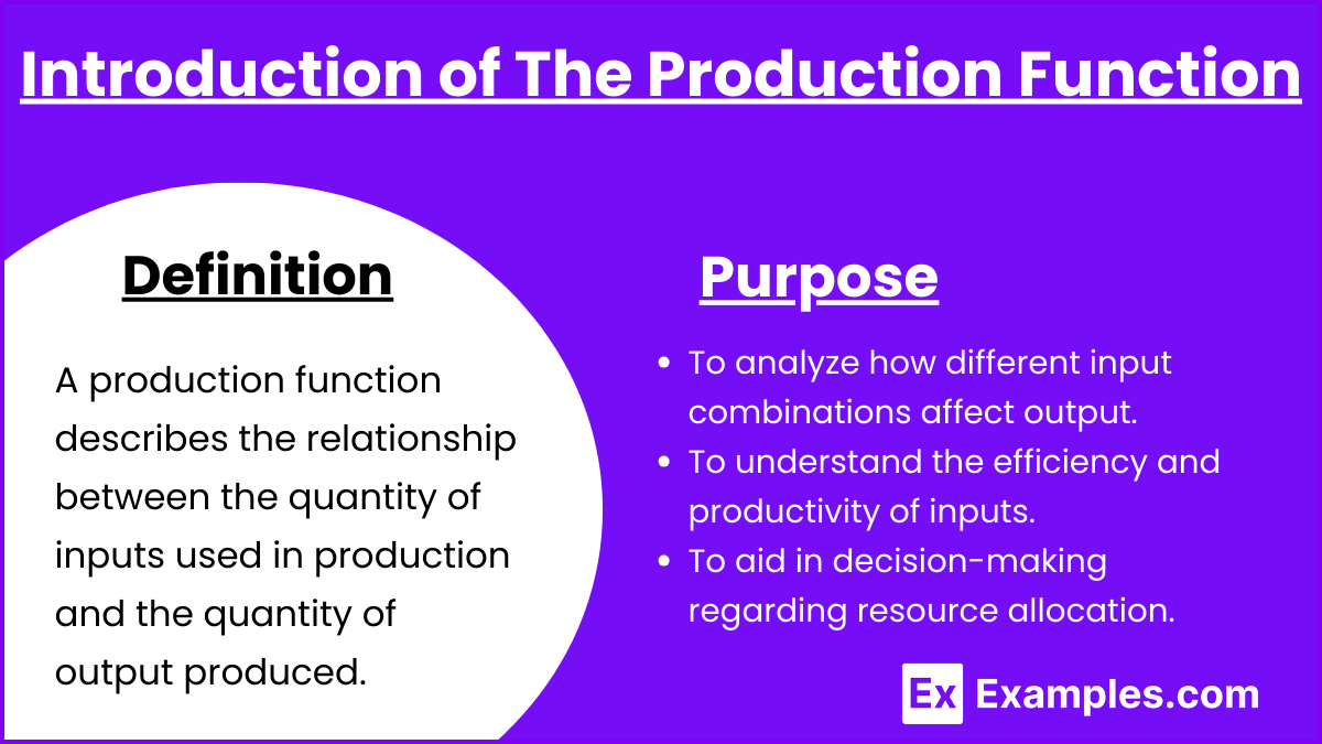
Definition: A production function describes the relationship between the quantity of inputs used in production and the quantity of output produced. It shows the maximum output that can be produced with a given set of inputs and the available technology.

Purpose:

To analyze how different input combinations affect output.
To understand the efficiency and productivity of inputs.
To aid in decision-making regarding resource allocation.

2. Components of the Production Function

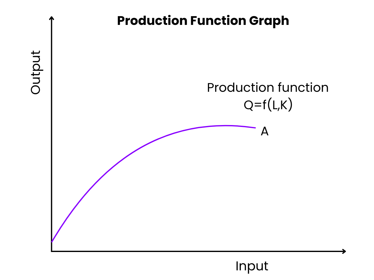
Inputs (Factors of Production):

Labor (L): Human effort used in production.
Capital (K): Machinery, tools, buildings, and other man-made resources.
Land (T): Natural resources used in production.
Entrepreneurship (E): The initiative to combine other factors of production to produce goods and services.

Note: In many basic models, capital and labor are the primary focus.

Output (Q):

The quantity of goods or services produced.

Mathematical Representation: Q=f(L,K) Where:

Q = Quantity of output
L = Quantity of labor
K = Quantity of capital

3. Types of Production Functions

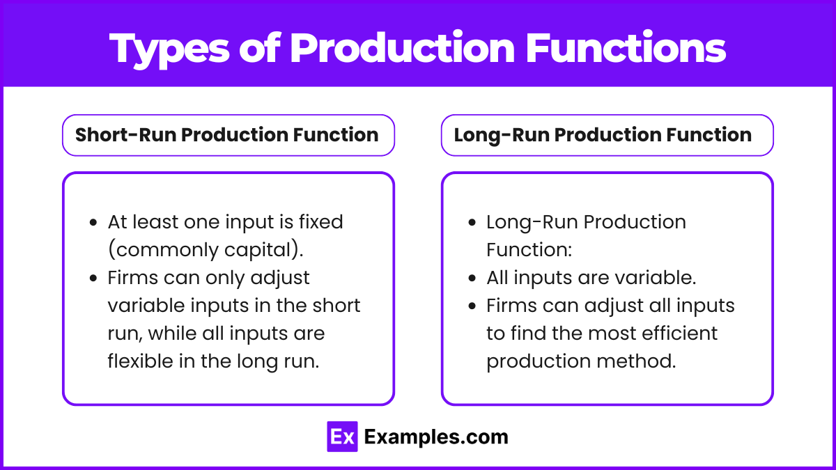
Short-Run vs. Long-Run:

Short-Run Production Function:
- At least one input is fixed (commonly capital).
- Firms can only adjust variable inputs (like labor) in the short run, while all inputs are flexible in the long run.
Long-Run Production Function:
- All inputs are variable.
- Firms can adjust all inputs to find the most efficient production method.

4. Law of Variable Proportions

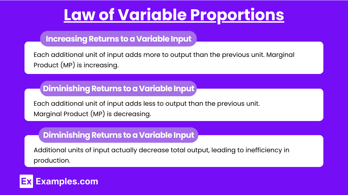
Concept: In the short run, as more of a variable input (e.g., labor) is added to fixed inputs (e.g., capital), the additional output produced by each additional unit of the variable input will eventually decrease.

Stages:

Increasing Returns to a Variable Input:
- Each additional unit of input adds more to output than the previous unit.
- Marginal Product (MP) is increasing.
Diminishing Returns to a Variable Input:
- Each additional unit of input adds less to output than the previous unit.
- Marginal Product (MP) is decreasing.
Negative Returns to a Variable Input:
- Additional units of input actually decrease total output.

Diagram Description: Imagine a graph with labor (L) on the horizontal axis and output (Q) on the vertical axis. The Total Product (TP) curve initially rises at an increasing rate, then continues to rise but at a decreasing rate, and may eventually decline.

5. Marginal Product (MP), Total Product (TP), and Average Product (AP)

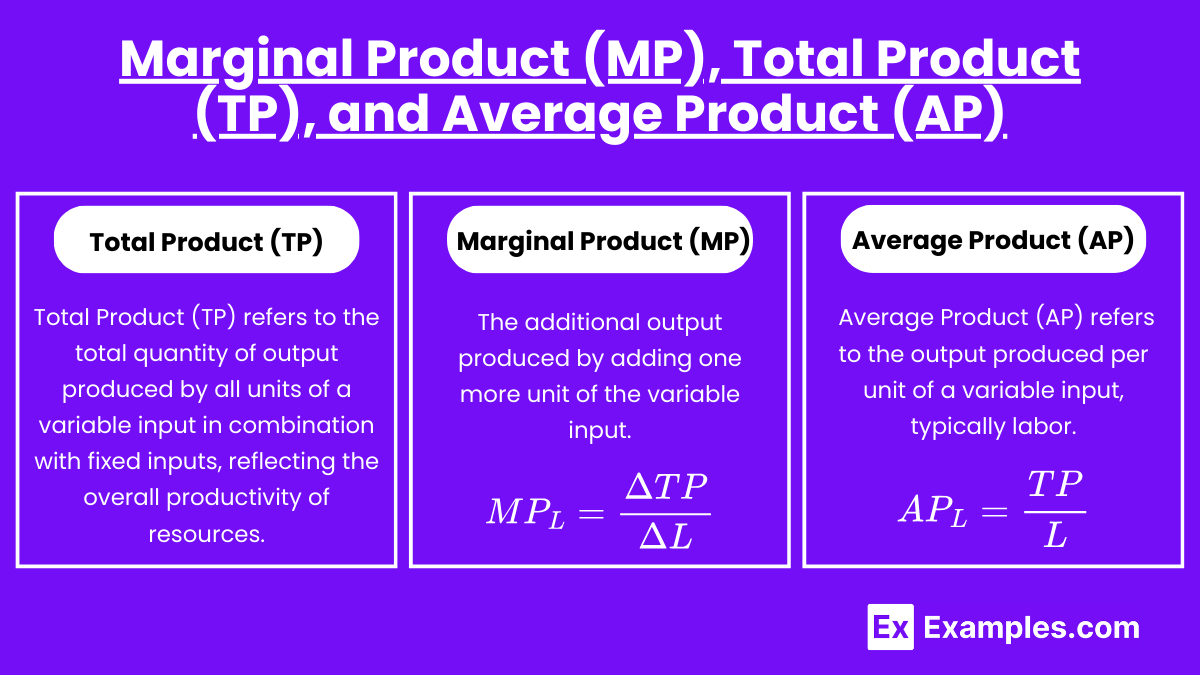
Total Product (TP):

The total quantity of output produced by all units of a variable input. Total Product (TP) refers to the total quantity of output produced by all units of a variable input in combination with fixed inputs, reflecting the overall productivity of resources.

Marginal Product (MP):

The additional output produced by adding one more unit of the variable input.
Formula: $MP_L = \frac{\Delta TP}{\Delta L}$

Average Product (AP):

The output produced per unit of the variable input. Average Product (AP) refers to the output produced per unit of a variable input, typically labor. It is calculated by dividing the total product (output) by the quantity of the input used.
Formula: $AP_L = \frac{TP}{L}$

Relationships:

When AP is rising, MP is above AP.
When AP is falling, MP is below AP.
The AP is maximized when MP=AP.

Examples

Example 1. Cobb-Douglas Production Function in Manufacturing

In the manufacturing sector, firms often use the Cobb-Douglas production function to model the relationship between inputs and output. For instance, consider a car manufacturing company that uses labor (L) and capital (K) as inputs to produce cars (Q). The production function can be represented as Q = A⋅L^α⋅K^β, where A is total factor productivity, and α and β are the output elasticities of labor and capital, respectively. This function assumes that output is a product of labor and capital raised to constant powers, reflecting the percentage change in output resulting from a percentage change in inputs. It illustrates how the firm can substitute between labor and capital while maintaining the same level of production, and it can exhibit constant, increasing, or decreasing returns to scale depending on the values of α and β.

Example 2. Leontief (Fixed Proportions) Production Function in Agriculture

An agricultural farm might operate under a Leontief production function, which assumes that inputs are used in fixed proportions. For example, a wheat farm requires a specific ratio of land (K) and labor (L) to produce wheat (Q). The production function is expressed as $Q = \min\left(\frac{L}{a}, \frac{K}{b}\right),$ , where a and b are fixed input coefficients. This means that adding more labor without increasing land does not increase output and vice versa. The function reflects situations where inputs are perfect complements, emphasizing the importance of using inputs in precise ratios. It is particularly relevant in agriculture, where certain resources like land cannot be easily substituted or scaled in the short run.

Example 3. Linear Production Function in Service Industry

In some service industries, such as freelance graphic design, the production function can be linear, indicating constant returns to scale. Suppose a graphic design firm measures output (Q) as the number of completed projects, with labor (L) as the primary input. The production function is Q = aL, where aaa represents the average productivity per designer. This linear relationship implies that each additional designer contributes the same amount of output, assuming equal skill levels and efficiency. The simplicity of the linear production function makes it useful for small firms to plan and predict how changes in labor input directly affect output, without the complexities of diminishing returns or input substitution.

Example 4. Increasing Returns to Scale in Technology Firms

Technology companies, such as software developers, often experience increasing returns to scale due to high fixed costs and low marginal costs. Consider a software company where the initial development (capital investment, K) is substantial, but the cost of distributing additional copies is minimal. The production function might be Q = A ⋅ (L + K)^γ with γ > 1, indicating that doubling inputs more than doubles output. This reflects economies of scale, where the average cost per unit decreases as production scales up. The production function demonstrates how tech firms benefit from spreading fixed costs over a larger output, leading to competitive advantages and potential market dominance.

Example 5. Decreasing Returns to Scale in Artisanal Crafting

In artisanal crafting businesses, such as handmade pottery studios, firms may encounter decreasing returns to scale. As the owner hires more artisans (labor, L) and adds more pottery wheels (capital, K), the production function Q = A⋅L^δ⋅K^δ with 0 < δ < 1 indicates that output increases at a diminishing rate. This occurs due to factors like limited space, coordination difficulties, and resource constraints. Each additional artisan contributes less to total output than the previous one. This production function highlights the challenges small businesses face when expanding, such as maintaining quality control and efficiency, and underscores the importance of optimal resource management.

Multiple Choice Questions

Question 1

The production function shows the relationship between:

A. Inputs and the price of goods
B. Inputs and the quantity of output produced
C. Labor costs and total revenue
D. Consumer preferences and production costs

Answer: B. Inputs and the quantity of output produced

Explanation: A production function expresses the relationship between the inputs used in production (such as labor, capital, land) and the quantity of output produced. It mathematically represents how much output a firm can produce given a specific amount of inputs. The goal of a production function is to understand how changes in input levels affect the output levels. It does not focus on prices, revenue, or consumer preferences, but solely on the efficiency of transforming inputs into outputs.

Question 2

In the short run, which of the following is true about the production function?

A. All inputs are variable
B. At least one input is fixed
C. The firm can freely adjust all resources
D. The firm is always operating at maximum efficiency

Answer: B. At least one input is fixed

Explanation: In the short run, a production function assumes that at least one input (such as capital) is fixed, meaning it cannot be changed quickly. For example, a firm cannot easily expand its factory size in the short run, but it can hire more labor or adjust raw material usage. The distinction between fixed and variable inputs defines the short-run production function. The firm cannot freely adjust all resources in the short run, which is only possible in the long run when all inputs can be varied.

Question 3

If the marginal product of labor is increasing, which of the following is true?

A. Total product is falling
B. Total product is increasing at an increasing rate
C. The marginal cost of production is increasing
D. Average product is zero

Answer: B. Total product is increasing at an increasing rate

Explanation: The marginal product of labor (MPL) refers to the additional output produced when one more unit of labor is employed. If the MPL is increasing, it means that each additional worker is adding more to total output than the previous one, causing total product to increase at an increasing rate. This typically happens in the early stages of production, where specialization and division of labor are at play. Eventually, due to the law of diminishing returns, MPL will start to decline, and total product will continue to rise, but at a decreasing rate.