Representations of Motion

Last Updated: November 7, 2024

Notes

Understanding the various representations of motion is essential for mastering AP Physics. These representations help visualize and analyze the movement of objects. Here are detailed notes to guide your study.

Free AP Physics 1: Algebra-Based Practice Test

Learning Objectives

By studying Representations of Motion for the AP Physics exam, you should learn to interpret and analyze position-time, velocity-time, and acceleration-time graphs, understand the relationship between these graphs, and use them to describe motion. You should also master motion diagrams, comprehend the significance of slopes and areas under curves, and apply kinematic equations to solve motion problems. These skills will enable you to visualize and quantify the motion of objects effectively, preparing you for various kinematics questions on the exam.

Graphical Representations

Position-Time Graphs

Key Points:

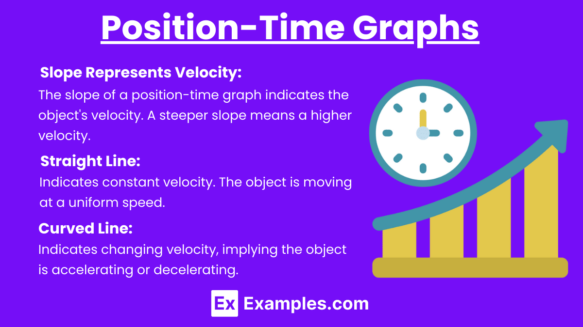
Slope Represents Velocity: The slope of a position-time graph indicates the object’s velocity. A steeper slope means a higher velocity.
Straight Line: Indicates constant velocity. The object is moving at a uniform speed.
Curved Line: Indicates changing velocity, implying the object is accelerating or decelerating.

Example:

A straight, diagonal line indicates constant velocity.
A parabolic curve indicates constant acceleration.

Velocity-Time Graphs

Key Points:

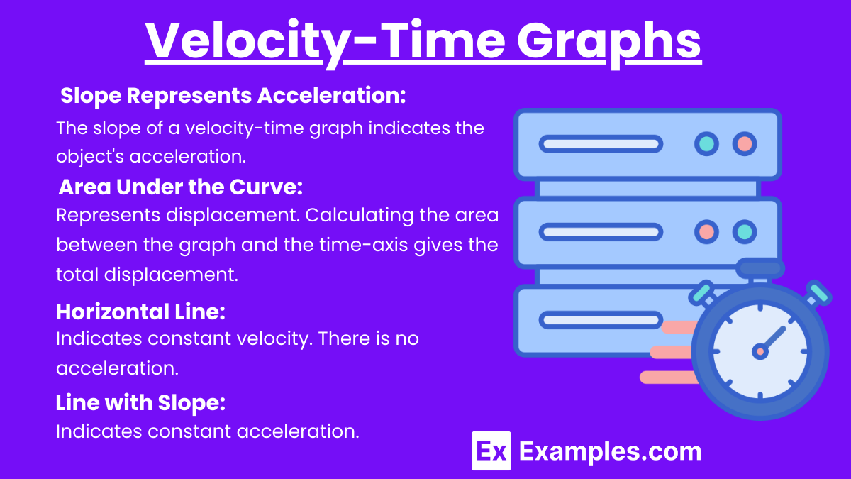
Slope Represents Acceleration: The slope of a velocity-time graph indicates the object’s acceleration.
Area Under the Curve: Represents displacement. Calculating the area between the graph and the time-axis gives the total displacement.
Horizontal Line: Indicates constant velocity. There is no acceleration.
Line with Slope: Indicates constant acceleration.

Example:

A horizontal line at v = 5 m/s indicates constant velocity.
A line with a positive slope indicates constant acceleration.

Acceleration-Time Graphs

Key Points:

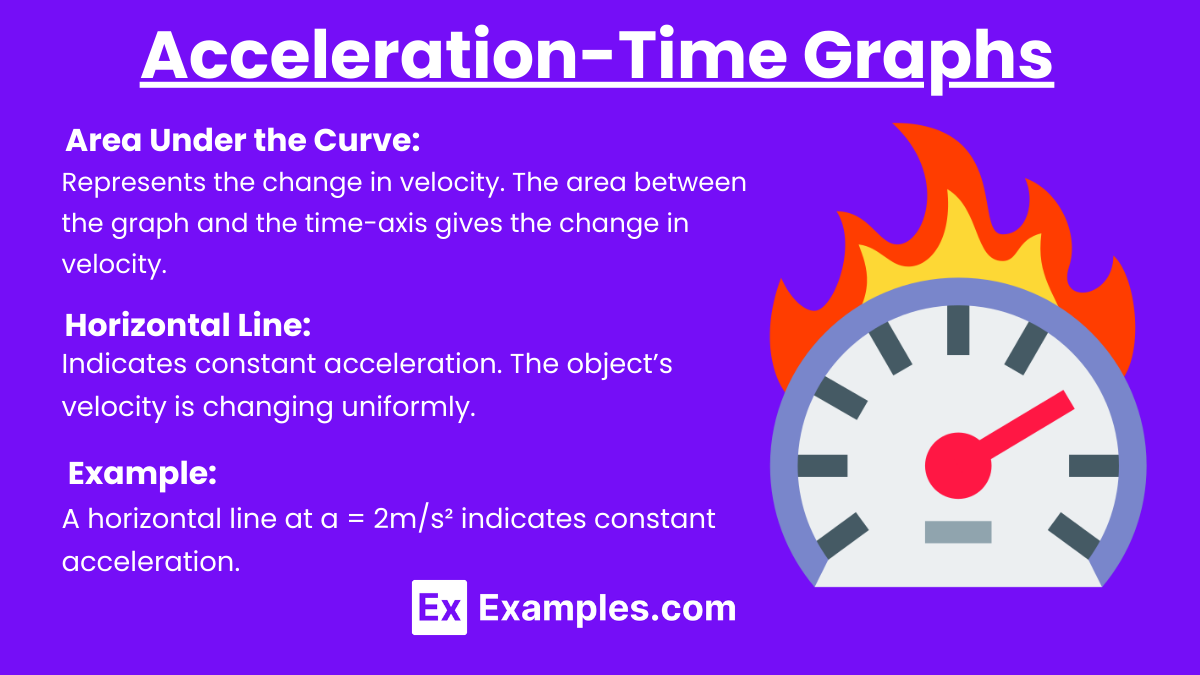
Area Under the Curve: Represents the change in velocity. The area between the graph and the time-axis gives the change in velocity.
Horizontal Line: Indicates constant acceleration. The object’s velocity is changing uniformly.

Example:

A horizontal line at a = 2m/s² indicates constant acceleration.

Motion Diagrams

Key Points:

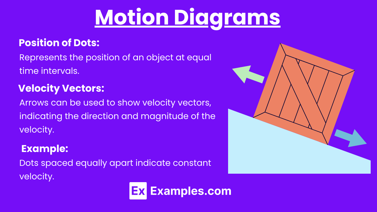
Position of Dots: Represents the position of an object at equal time intervals. The spacing of the dots indicates the speed of the object (closer dots mean slower speed; wider dots mean faster speed).
Velocity Vectors: Arrows can be used to show velocity vectors, indicating the direction and magnitude of the velocity.

Example:

Dots spaced equally apart indicate constant velocity.
Increasing space between dots indicates acceleration.

Mathematical Representations

Kinematic Equations:

For constant acceleration, the following equations are used:

$v = v_0 + at$

$x = x_0 + v_0 t + \frac{1}{2} at^2$

$v^2 = v_0^2 + 2a(x - x_0)$

$x = x_0 + \frac{1}{2}(v + v_0)t$

Key Points:

These equations relate displacement (x), initial velocity (v₀), final velocity (v), acceleration (a), and time (t).
They are derived from the definitions of velocity and acceleration.

Examples

Example 1: Interpreting a Position-Time Graph

Given a position-time graph where the line is straight and diagonal:

Interpretation: The object is moving with constant velocity.
Slope Calculation: The slope of the line gives the velocity of the object.

Example 2: Analyzing a Velocity-Time Graph

Given a velocity-time graph with a line that slopes upwards:

Interpretation: The object is accelerating.
Slope Calculation: The slope of the line gives the acceleration.
Area Calculation: The area under the line gives the displacement.