
Vector and Scalar Fields

![\[ \nabla \phi = \frac{\partial \phi}{\partial x} \hat{i} + \frac{\partial \phi}{\partial y} \hat{j} + \frac{\partial \phi}{\partial z} \hat{k} \]](https://www.examples.com/wp-content/ql-cache/quicklatex.com-ae8203efb0944ed8e51c0a8e172ffe1d_l3.svg "Rendered by QuickLaTeX.com")
![\[ \nabla \phi = 2x \hat{i} + 2y \hat{j} + 2z \hat{k} \]](https://www.examples.com/wp-content/ql-cache/quicklatex.com-42f15a7fa5e7e5bf5411e3828ae7490e_l3.svg "Rendered by QuickLaTeX.com")
![\[ \nabla \cdot \mathbf{F} = \frac{\partial F_x}{\partial x} + \frac{\partial F_y}{\partial y} + \frac{\partial F_z}{\partial z} \]](https://www.examples.com/wp-content/ql-cache/quicklatex.com-81c89f02786cc8806b1277499e0f03fd_l3.svg "Rendered by QuickLaTeX.com")
 then the divergence is:
![\[ \nabla \cdot \mathbf{F} = \frac{\partial x}{\partial x} + \frac{\partial y}{\partial y} + \frac{\partial z}{\partial z} = 1 + 1 + 1 = 3 \]](https://www.examples.com/wp-content/ql-cache/quicklatex.com-b45dd74c99c84d79953f1ec64380c17f_l3.svg "Rendered by QuickLaTeX.com")
![\[ \nabla \times \mathbf{F} = \left( \frac{\partial F_z}{\partial y} - \frac{\partial F_y}{\partial z} \right) \hat{i} + \left( \frac{\partial F_x}{\partial z} - \frac{\partial F_z}{\partial x} \right) \hat{j} + \left( \frac{\partial F_y}{\partial x} - \frac{\partial F_x}{\partial y} \right) \hat{k} \]](https://www.examples.com/wp-content/ql-cache/quicklatex.com-370a2d66497859f384dd4507f9ad14f1_l3.svg "Rendered by QuickLaTeX.com")
 then the curl is:
![\[ \nabla \times \mathbf{F} = \left( \frac{\partial 0}{\partial y} - \frac{\partial z}{\partial z} \right) \hat{i} + \left( \frac{\partial (-y)}{\partial z} - \frac{\partial 0}{\partial x} \right) \hat{j} + \left( \frac{\partial x}{\partial x} - \frac{\partial (-y)}{\partial y} \right) \hat{k} = 0 \hat{i} + 0 \hat{j} + (1 - (-1)) \hat{k} = 2 \hat{k} \]](https://www.examples.com/wp-content/ql-cache/quicklatex.com-2cdab8935581e2782269b0a34fd09c47_l3.svg "Rendered by QuickLaTeX.com")
Understanding vector and scalar fields is crucial. A scalar field assigns a magnitude to every point in space, while a vector field assigns both magnitude and direction. Key concepts include gradient, divergence, and curl, which help describe how fields change over space. Applications span across electromagnetism and fluid dynamics, making these concepts fundamental in AP Physics. Mastery of these topics involves visualization, and problem-solving using field diagrams and physical interpretations.
Free AP Physics 2: Algebra-Based Practice Test
Learning Objectives
Focus on understanding the definitions and differences between scalar and vector fields. Study the concepts of gradient, divergence, and curl, and how to compute them. Apply these principles to solve problems in electromagnetism and fluid dynamics. Develop skills in interpreting and drawing field diagrams, and understand the physical significance of these fields in various physical contexts.
Fields
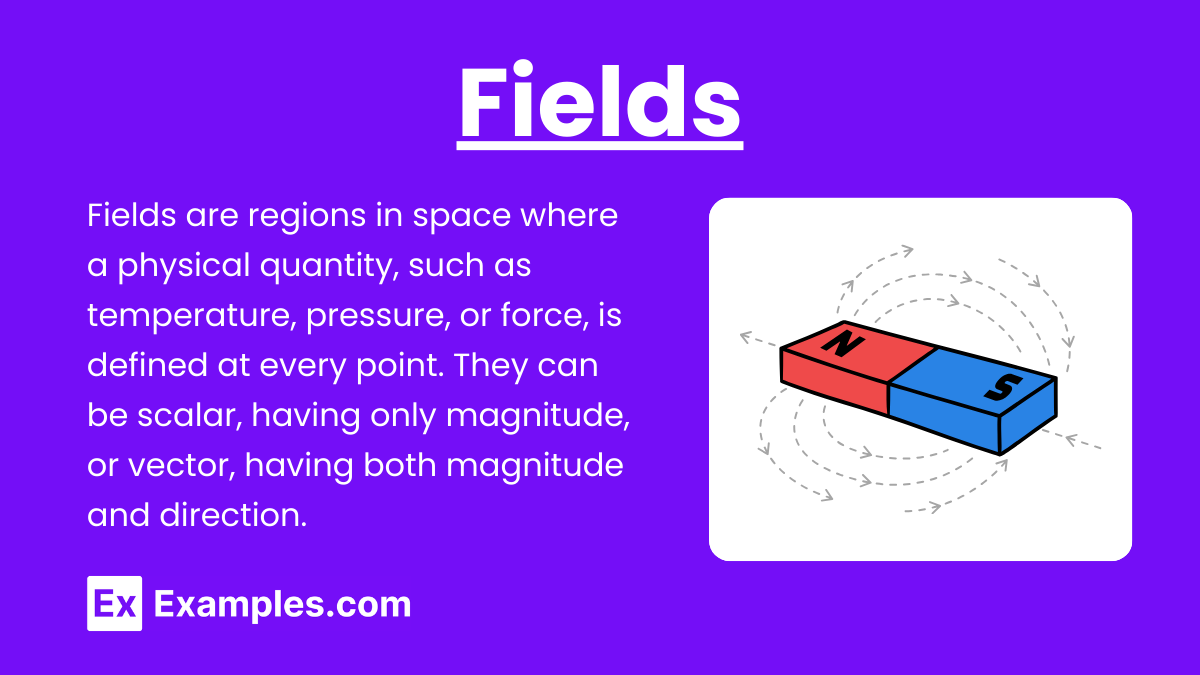
A field is a region of space where a physical quantity can be measured at every point. Fields are used to describe the distribution of forces and other physical quantities in space.
Scalar Fields
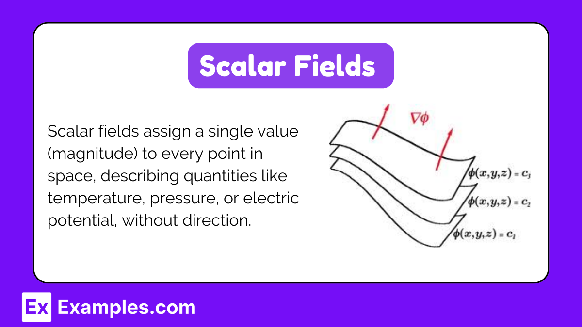
A scalar field is a field that associates a scalar value (a single number) with every point in space. Scalar fields are often used to describe quantities that only have magnitude and no direction.
Examples of Scalar Fields
Temperature Field: The temperature at every point in a room can be described by a scalar field.
Pressure Field: The atmospheric pressure at different points on Earth forms a scalar field.
Electric Potential Field: The electric potential in the space around a charged object is a scalar field.
Visualization
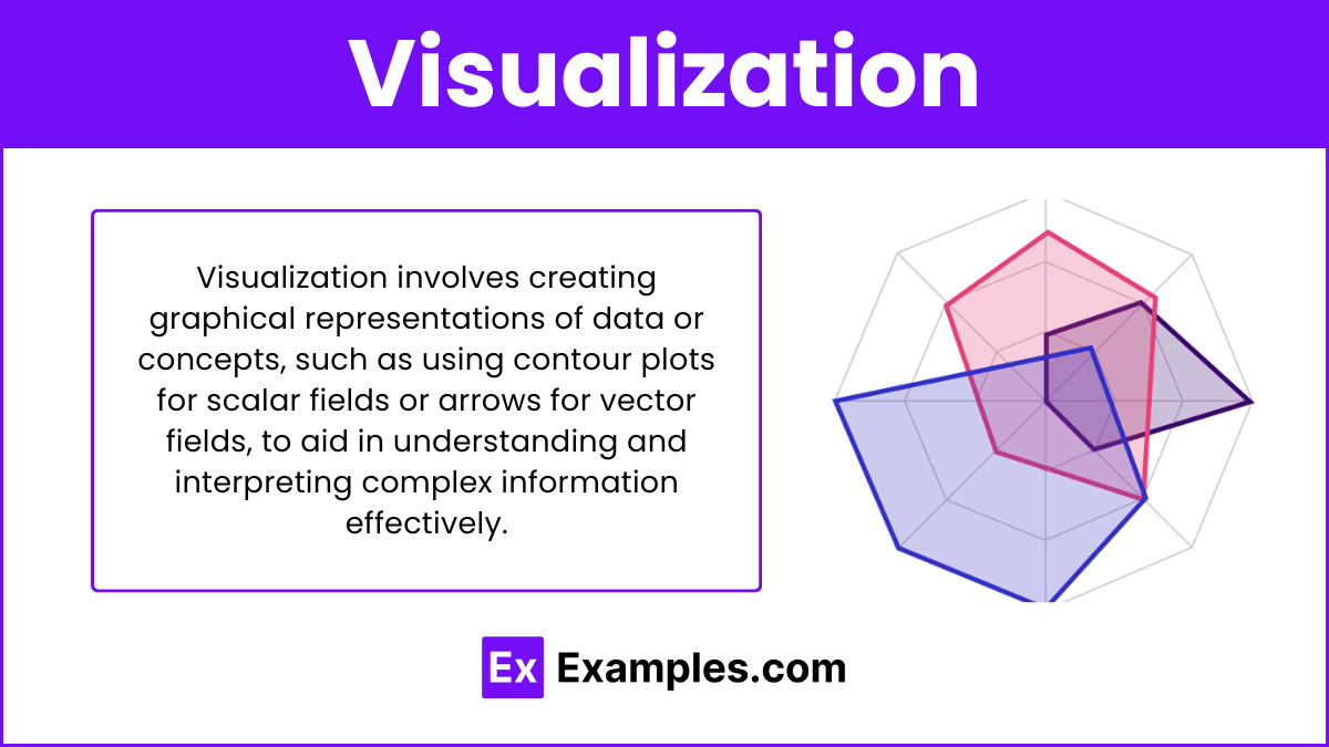
Scalar fields can be visualized using contour plots or color maps, where each color or contour line represents a different scalar value.
Vector Fields
A vector field is a field that associates a vector (having both magnitude and direction) with every point in space. Vector fields are used to describe quantities that have both magnitude and direction.
Examples of Vector Fields
Gravitational Field: The gravitational force experienced by a mass at any point in space.
Electric Field: The force experienced by a charge at any point in space.
Velocity Field: The velocity of fluid particles at different points in a flow field.
Visualization
Vector fields can be visualized using arrows (vectors) at various points in space, where the direction and length of the arrow represent the direction and magnitude of the vector at that point.
Key Differences Between Scalar and Vector Fields
Property | Scalar Field | Vector Field |
|---|---|---|
Quantity Described | Scalar (magnitude only) | Vector (magnitude and direction) |
Representation | ϕ(x,y,z) | F(x,y,z) |
Examples | Temperature, Pressure, Electric Potential | Gravitational Field, Electric Field, Velocity Field |
Visualization | Contour plots, color maps | Arrows, vector plots |
Applications
Scalar Fields
Electrostatics: The electric potential field helps in understanding the work done in moving a charge in an electric field.
Thermodynamics: Temperature fields are crucial for studying heat distribution and transfer.
Vector Fields
Mechanics: Gravitational and electric fields explain forces acting on masses and charges, respectively.
Fluid Dynamics: Velocity fields describe the movement of fluids and are essential for analyzing fluid flow patterns.
Gradient of a Scalar Field
The gradient of a scalar field ϕ(x,y,z) is a vector field that points in the direction of the greatest rate of increase of the scalar field. It is denoted by ∇ϕ is given by:
\nabla \phi = \frac{\partial \phi}{\partial x} \hat{i} + \frac{\partial \phi}{\partial y} \hat{j} + \frac{\partial \phi}{\partial z} \hat{k}
Example
If ϕ(x,y,z)=x²+y²+z² then the gradient is:
\nabla \phi = 2x \hat{i} + 2y \hat{j} + 2z \hat{k}
Divergence of a Vector Field
The divergence of a vector field F(x,y,z) measures the rate at which "density" exits a point. It is denoted by ∇⋅F is given by:
\nabla \cdot \mathbf{F} = \frac{\partial F_x}{\partial x} + \frac{\partial F_y}{\partial y} + \frac{\partial F_z}{\partial z}
Example
If F(x,y,z)= then the divergence is:
\nabla \cdot \mathbf{F} = \frac{\partial x}{\partial x} + \frac{\partial y}{\partial y} + \frac{\partial z}{\partial z} = 1 + 1 + 1 = 3
Curl of a Vector Field
The curl of a vector field F(x,y,z) measures the rotation or the "circulation" of the field around a point. It is denoted by ∇×F is given by:
\nabla \times \mathbf{F} = \left( \frac{\partial F_z}{\partial y} - \frac{\partial F_y}{\partial z} \right) \hat{i} + \left( \frac{\partial F_x}{\partial z} - \frac{\partial F_z}{\partial x} \right) \hat{j} + \left( \frac{\partial F_y}{\partial x} - \frac{\partial F_x}{\partial y} \right) \hat{k}
Example
If F(x,y,z)= then the curl is:
\nabla \times \mathbf{F} = \left( \frac{\partial 0}{\partial y} - \frac{\partial z}{\partial z} \right) \hat{i} + \left( \frac{\partial (-y)}{\partial z} - \frac{\partial 0}{\partial x} \right) \hat{j} + \left( \frac{\partial x}{\partial x} - \frac{\partial (-y)}{\partial y} \right) \hat{k} = 0 \hat{i} + 0 \hat{j} + (1 - (-1)) \hat{k} = 2 \hat{k}