

Fields and Potentials of other Charge Distributions

In AP Physics, understanding the fields and potentials of various charge distributions is essential for mastering electrostatics. Charge distributions can vary widely, from point charges to continuous distributions such as line, surface, and volume charges. Each type of distribution creates unique electric fields and potentials that influence how charges interact in space. By exploring these different charge configurations, students gain deeper insights into the principles of electric fields and potentials, which are critical for solving complex problems in electrostatics.
Learning Objectives
For the AP Physics exam, you should learn how to calculate electric fields and potentials for various continuous charge distributions, including line, surface, and volume charges. Understand the application of Coulomb’s law and Gauss’s law in deriving these fields and potentials. Focus on solving problems involving infinite line charges, charged planes, and uniformly charged spheres. Develop proficiency in integrating charge distributions to find electric fields and potentials. Grasp the physical significance of these concepts and their applications in real-world scenarios.
Continuous Charge Distributions
Line Charge Distribution
A line charge is a continuous distribution of charge along a line, characterized by a linear charge density λ\lambdaλ (charge per unit length).
Electric Field of a Line Charge
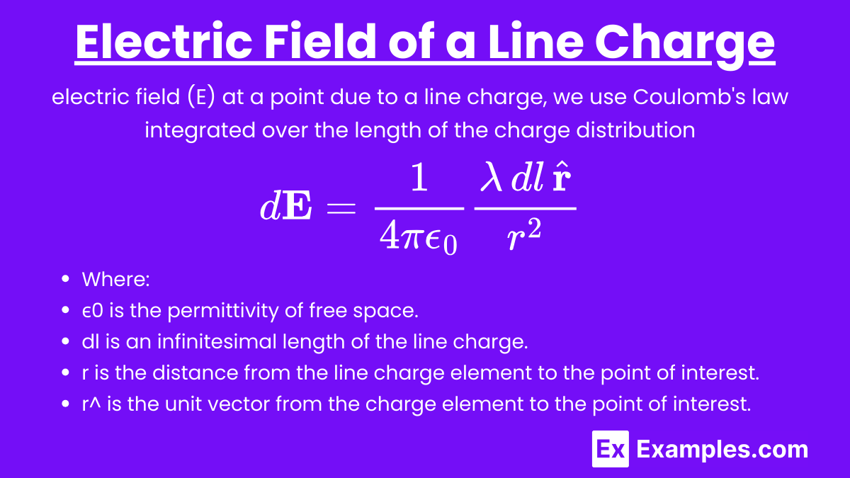
To find the electric field (E) at a point due to a line charge, we use Coulomb’s law integrated over the length of the charge distribution:

Where:
- ϵ0 is the permittivity of free space.
- dl is an infinitesimal length of the line charge.
- r is the distance from the line charge element to the point of interest.
- r^ is the unit vector from the charge element to the point of interest.
For a line charge of infinite length, the electric field at a distance rrr from the line is:

This field points radially outward from the line if the charge is positive, and radially inward if the charge is negative.
Potential of a Line Charge
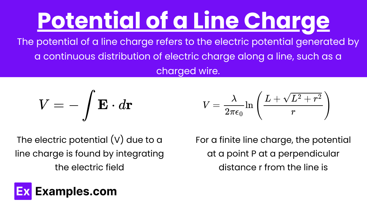
The potential of a line charge refers to the electric potential generated by a continuous distribution of electric charge along a line, such as a charged wire. It is a measure of the work done to bring a unit positive charge from infinity to a point in the vicinity of the line charge without any acceleration.
The electric potential (V) due to a line charge is found by integrating the electric field:

For a finite line charge, the potential at a point P at a perpendicular distance r from the line is:

Where L is half the length of the line charge.
Surface Charge Distribution
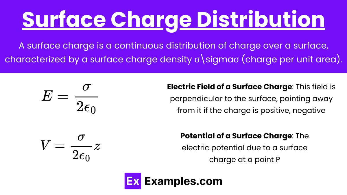
A surface charge is a continuous distribution of charge over a surface, characterized by a surface charge density σ\sigmaσ (charge per unit area).
Electric Field of a Surface Charge
For a surface charge, the electric field just above and below the surface can be found using Gauss’s law. For a large, flat surface with charge density σ:

This field is perpendicular to the surface, pointing away from it if the charge is positive, and toward it if the charge is negative.
Potential of a Surface Charge
The electric potential due to a surface charge at a point P is:

Where z is the perpendicular distance from the surface to the point P.
Volume Charge Distribution
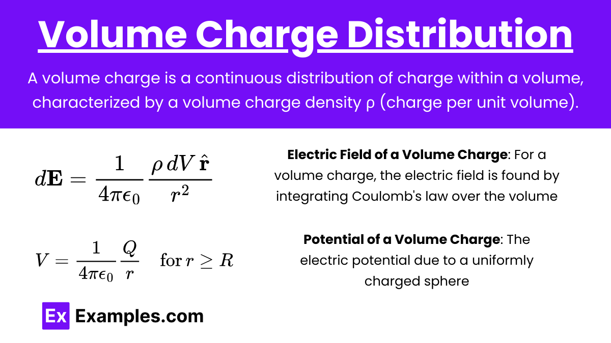
A volume charge is a continuous distribution of charge within a volume, characterized by a volume charge density ρ (charge per unit volume).
Electric Field of a Volume Charge
For a volume charge, the electric field is found by integrating Coulomb’s law over the volume:

Where dV is an infinitesimal volume element.
For a uniformly charged sphere with total charge Q and radius R, the electric field outside the sphere (r>R) is:

Inside the sphere (r≤Rr), the field is:

Potential of a Volume Charge
The electric potential due to a uniformly charged sphere is:


Examples
Example 1. Uniformly Charged Ring
A uniformly charged ring with total charge Q and radius R lying in the xy-plane with its center at the origin.
Electric Potential:

Electric Field:

Example 2. Infinite Line Charge
An infinitely long line charge with linear charge density λ.
Electric Potential:

Where r0 is a reference distance.
Electric Field:

Example 3. Uniformly Charged Disk
A uniformly charged disk with surface charge density σ and radius R lying in the xy-plane.
Electric Potential (on the axis):

Electric Field (on the axis):

Example 4. Spherical Shell
A thin spherical shell with radius R uniformly charged with total charge Q.
Electric Potential:
- Inside the shell (r < R):

- Outside the shell (r \geq R):

Electric Field:
- Inside the shell (r < R):

- Outside the shell (r \geq R):

Example 5. Dipole Field
An electric dipole consisting of two opposite charges +q and −q separated by a distance d.
Electric Potential:

Where p=qd is the dipole moment.
Electric Field:

Multiple Choice Questions
1. Which of the following correctly describes the electric potential V at a point due to a continuous charge distribution?
a) 
b) 
c) 
d)  ′
′
Answer: b)
Explanation: The electric potential V at a point due to a continuous volume charge distribution is given by where ( \rho(\mathbf{r}’) is the charge density at position ( \mathbf{r}’ ), and ( |\mathbf{r} – \mathbf{r}’| )is the distance between the point where the potential is being calculated and the location of the charge element dV′. This formula is derived from the principle of superposition and Coulomb’s law for a continuous charge distribution.
2. What is the electric field E at a distance r from an infinitely long line of charge with linear charge density λ?
a) 
b) 
c) 
d)
Answer: a)
Explanation: The electric field E at a distance rrr from an infinitely long line of charge with linear charge density λ is given by This result is obtained by applying Gauss’s law to a cylindrical Gaussian surface co-axial with the line of charge. The symmetry of the problem indicates that the electric field will be radial and will have the same magnitude at every point equidistant from the line of charge.
3. For a spherical shell of radius R carrying a uniform surface charge density σ, what is the electric potential VVV at a distance rrr from the center, where r<R?
a) 
b) 
c)
d) 
Answer: c)
Explanation: Inside a spherical shell of radius R with uniform surface charge density σ\sigmaσ, the electric potential V at a distance rrr from the center, where r<Rr, is given by This result comes from the fact that inside a spherical shell, the electric field is zero (by Gauss’s law), and the potential inside the shell is constant and equal to the potential on the surface. The potential on the surface is given by integrating the potential contributions from all the infinitesimal surface charges.