
Maxwell’s Equations

Maxwell’s Equations are the cornerstone of electromagnetism, describing how electric and magnetic fields interact and propagate. These four equations—Gauss’s Law for Electricity, Gauss’s Law for Magnetism, Faraday’s Law of Induction, and Ampère’s Law with Maxwell’s addition—are essential for understanding the behavior of electromagnetic fields. In AP Physics, mastering these equations is crucial for solving problems related to electric and magnetic fields, wave propagation, and their practical applications in technology.
Learning Objectives
Understand and apply Maxwell’s Equations: Gauss’s Law for Electricity, Gauss’s Law for Magnetism, Faraday’s Law of Induction, and Ampère’s Law with Maxwell’s addition. Focus on their mathematical forms, physical meanings, and implications for electric and magnetic fields. Practice solving problems involving these equations, including calculating electric and magnetic fields, understanding electromagnetic wave propagation, and recognizing their applications in real-world phenomena and technology.
Maxwell’s Equations
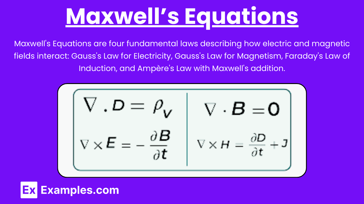
Maxwell’s Equations are a set of four fundamental laws that form the foundation of classical electromagnetism, electrodynamics, and electric circuits. They describe how electric and magnetic fields are generated and altered by each other and by charges and currents. These equations are essential for understanding various physical phenomena and technologies.
1. Gauss’s Law for Electricity
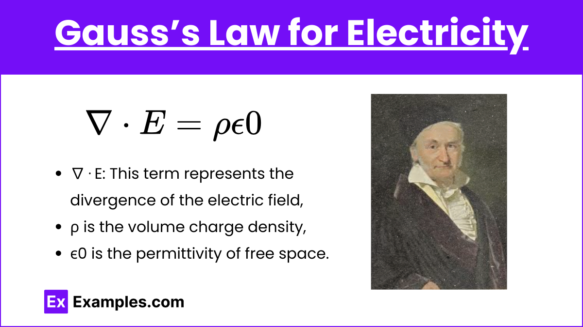
Equation: 
Description: Gauss’s Law states that the electric flux through a closed surface is proportional to the charge enclosed within that surface. It implies that electric charges produce an electric field.
Key Concepts:
- Electric Flux (ΦE): The amount of electric field passing through a surface.
- Charge Density (ρ): Amount of charge per unit volume.
- Permittivity of Free Space (ϵ0): A constant that characterizes the strength of the electric field in a vacuum.
2. Gauss’s Law for Magnetism
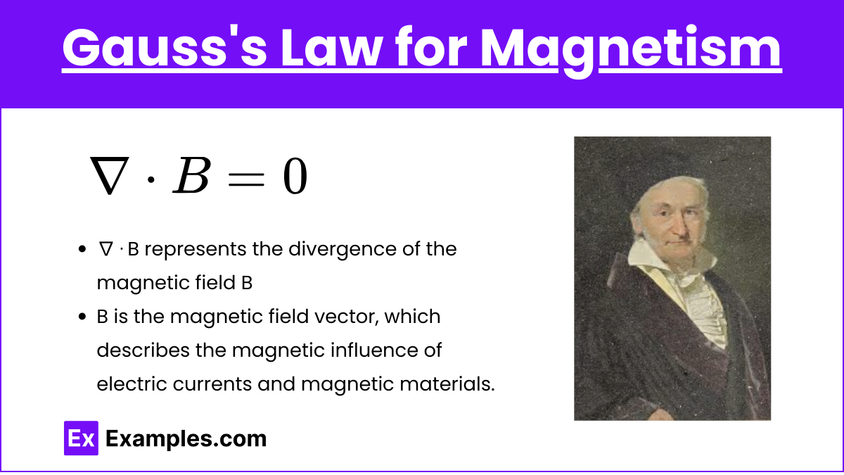
Equation: ∇⋅B=0
Description: Gauss’s Law for Magnetism states that the magnetic flux through a closed surface is zero. This implies that there are no magnetic monopoles; magnetic field lines are continuous loops.
Key Concepts:
- Magnetic Flux (ΦB): The amount of magnetic field passing through a surface.
- Magnetic Field (B): A vector field that represents the magnetic influence on moving electric charges.
3. Faraday’s Law of Induction
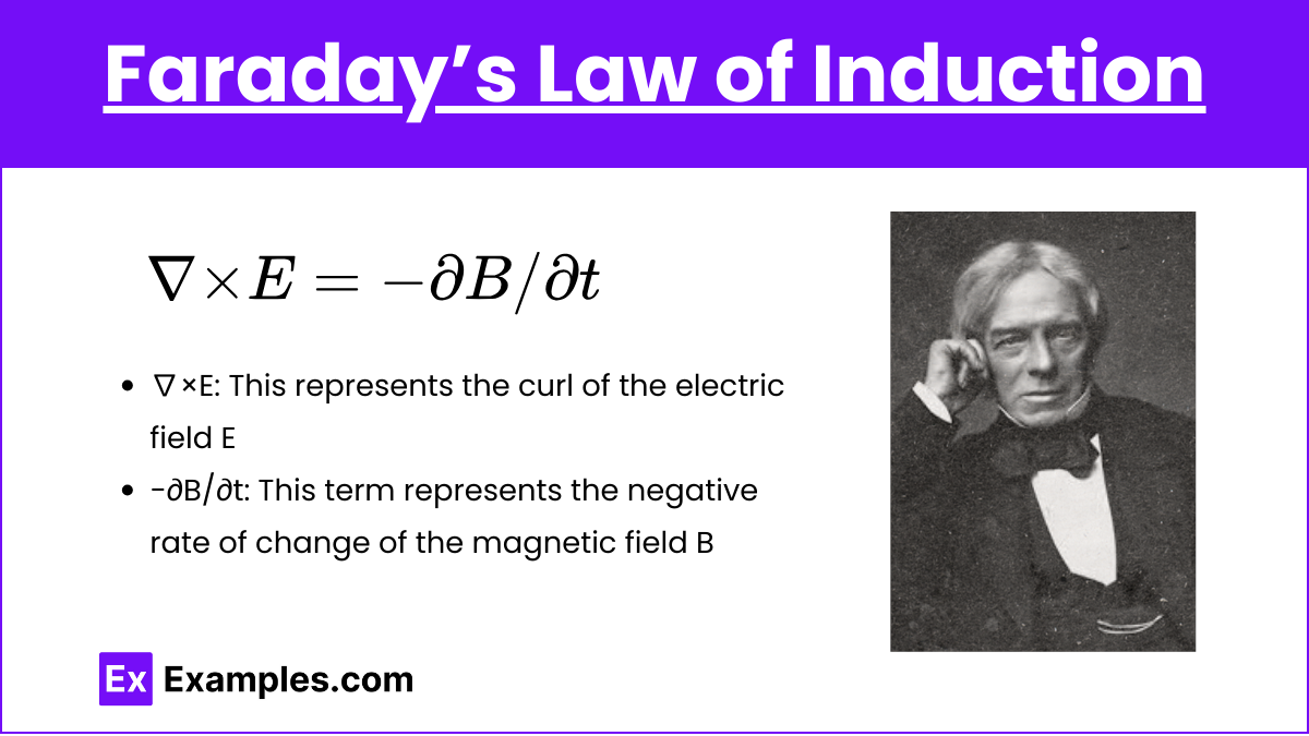
Equation: 
Description: Faraday’s Law states that a changing magnetic field induces an electric field. This is the principle behind electric generators and transformers.
Key Concepts:
- Electromotive Force (EMF): The voltage generated by a changing magnetic field.
- Induced Electric Field (E): An electric field created by a time-varying magnetic field.
4. Ampère’s Law (with Maxwell’s Addition)
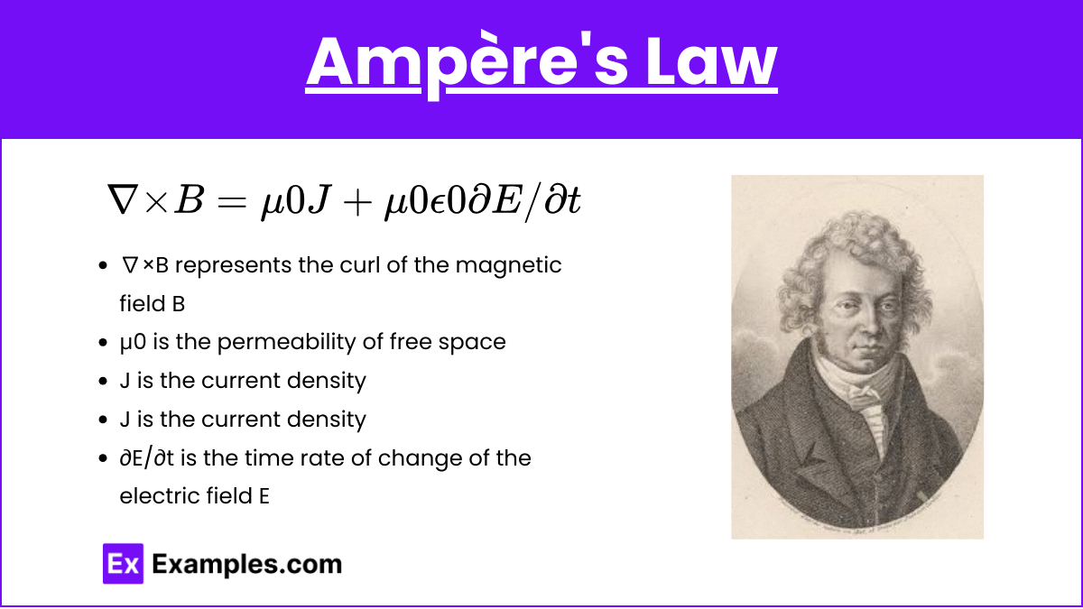
Equation: 
Description: Ampère’s Law relates magnetic fields to the electric currents and changing electric fields that produce them. Maxwell added the term  , accounting for the displacement current.
Key Concepts:
- Magnetic Field (B): Generated by electric currents and changing electric fields.
- Current Density (J): Amount of electric current per unit area.
- Permeability of Free Space (μ0): A constant that characterizes the strength of the magnetic field in a vacuum.
- Displacement Current: A term added by Maxwell to account for changing electric fields in regions without a physical current.
Applications and Implications
Electromagnetic Waves
Maxwell’s Equations predict the existence of electromagnetic waves, which propagate at the speed of light (c). These waves include radio waves, microwaves, infrared, visible light, ultraviolet, X-rays, and gamma rays.
Electromagnetic Spectrum
- Radio Waves: Used in communication (radio, TV).
- Microwaves: Used in cooking and radar.
- Infrared: Used in night vision and remote controls.
- Visible Light: The spectrum visible to the human eye.
- Ultraviolet: Causes sunburn; used in sterilization.
- X-rays: Used in medical imaging.
- Gamma Rays: Emitted by radioactive materials; used in cancer treatment.
Electromagnetic Wave Equation
From Maxwell’s Equations, we derive the wave equation for electric and magnetic fields:


Speed of Light
The speed of light ccc is related to the permittivity and permeability of free space:

Examples of Maxwell’s Equations
- Calculating Electric Field from a Point Charge (Gauss’s Law for Electricity)
- Use Gauss’s Law to determine the electric field surrounding a point charge by considering a spherical Gaussian surface.
- Magnetic Field Inside a Toroid (Gauss’s Law for Magnetism)
- Apply Gauss’s Law for Magnetism to show that the net magnetic flux through a closed surface inside a toroid is zero, indicating no magnetic monopoles.
- Induced EMF in a Rotating Loop (Faraday’s Law of Induction)
- Determine the electromotive force (EMF) induced in a loop of wire rotating in a magnetic field, demonstrating Faraday’s Law.
- Magnetic Field Around a Solenoid (Ampère’s Law with Maxwell’s Addition)
- Use Ampère’s Law to calculate the magnetic field inside a solenoid carrying a steady current, incorporating the displacement current term if the current changes.
- Propagation of Electromagnetic Waves (Combination of Maxwell’s Equations)
- Show how the equations predict the existence of electromagnetic waves traveling at the speed of light, with oscillating electric and magnetic fields perpendicular to each other.
Multiple Choice Questions on Maxwell’s Equations
Question 1: Which of the following Maxwell’s Equations states that the net magnetic flux through a closed surface is zero?
A)
B) 
C)
D)
Answer: B)
Explanation: This equation is Gauss’s Law for Magnetism, which states that there are no magnetic monopoles and that magnetic field lines form continuous loops. The net magnetic flux through any closed surface is zero, meaning magnetic field lines do not begin or end but instead loop through and around surfaces.
Question 2: Which of Maxwell’s Equations is used to describe how a changing magnetic field can induce an electric field?
A)
B)
C)
D)
Answer: C)
Explanation: Faraday’s Law of Induction describes how a time-varying magnetic field induces an electric field. This principle is fundamental in the operation of transformers, electric generators, and inductors, where a changing magnetic field generates an electromotive force (EMF).
Question 3: In which of the following scenarios is Ampère’s Law with Maxwell’s addition used?
A) Calculating the electric field of a point charge.
B) Determining the magnetic flux through a closed surface.
C) Finding the induced EMF in a loop due to a changing magnetic field.
D) Calculating the magnetic field in a capacitor with a time-varying electric field.
Answer: D) Calculating the magnetic field in a capacitor with a time-varying electric field.
Explanation: Ampère’s Law with Maxwell’s addition, , incorporates the displacement current term  . This term is crucial for scenarios where the electric field is changing over time, such as within a charging or discharging capacitor, ensuring continuity in the magnetic field calculation even in the absence of a physical current.