Describing How Quantities Change With Respect to Each Other

In AP Precalculus, understanding how quantities change with respect to each other is essential for analyzing various mathematical relationships. This concept involves examining the rate of change, whether it’s constant or variable, and how functions like linear, quadratic, and exponential express these changes. By interpreting graphs, formulas, and real-world scenarios, students learn to describe how one variable affects another. Mastering this concept is critical for solving problems related to motion, growth, economics, and many other applications in both mathematics and science.

Learning Objectives

In the topic “Describing How Quantities Change With Respect to Each Other” for AP Precalculus, you should focus on understanding and identifying different types of rate of change, such as constant, variable, average, and instantaneous rates. You should learn to interpret these changes in linear, quadratic, and exponential functions, both algebraically and graphically. Additionally, recognizing how these changes apply to real-world scenarios, such as velocity, economics, and population growth, is essential. You should also practice using functions to model and describe varying relationships between quantities.

In AP Precalculus, describing how quantities change with respect to each other is a fundamental concept related to understanding rates of change, functional relationships, and the behavior of various mathematical models. Here’s a detailed explanation to help you master this topic:

Understanding Rates of Change

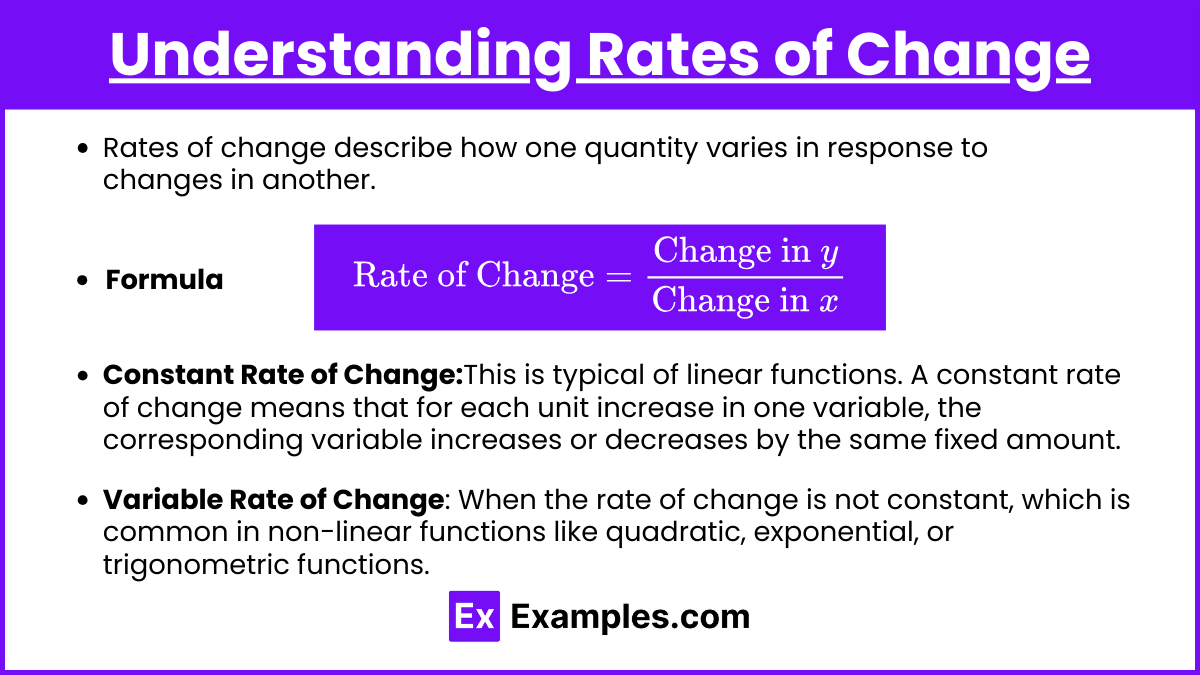
Rates of change describe how one quantity changes in response to another. Rates of change describe the relationship between two varying quantities, showing how one quantity changes in response to changes in another. Mathematically, it is often expressed as the ratio of the change in one quantity to the change in another.The two main types of change are:

The basic formula for the rate of change can be expressed as:

\(\text{Rate of Change} = \frac{\text{Change in } y}{\text{Change in } x} \)

• Constant Rate of Change: When a quantity increases or decreases by a fixed amount with respect to another quantity. This is typical of linear functions. A constant rate of change means that for each unit increase in one variable, the corresponding variable increases or decreases by the same fixed amount. This is characteristic of linear functions, where the relationship between two variables can be expressed as a straight line. The slope of this line represents the constant rate of change and remains unchanged over time.
• Variable Rate of Change: When the rate of change is not constant, which is common in non-linear functions like quadratic, exponential, or trigonometric functions. A variable rate of change occurs when the rate at which one quantity changes with respect to another is not constant. This is typical in non-linear functions, such as quadratic, exponential, logarithmic, and trigonometric functions. In these cases, the slope of the graph changes at different points.

Slope as a Measure of Rate of Change

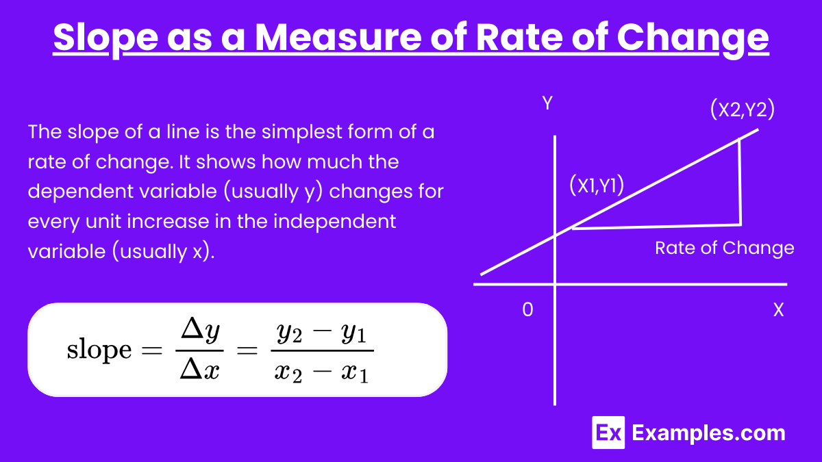
The slope of a line is the simplest form of a rate of change. It shows how much the dependent variable (usually y) changes for every unit increase in the independent variable (usually x). The formula for the slope is:

\(\text{slope} = \frac{\Delta y}{\Delta x} = \frac{y_2 – y_1}{x_2 – x_1} \)

For linear functions, this slope remains constant, indicating a constant rate of change.

Rates of Change in Non-Linear Functions

For non-linear functions, the rate of change varies. You can approximate it using average rate of change over an interval or instantaneous rate of change (which is connected to calculus concepts like derivatives).

Average Rate of Change: Between two points (x1​,y1​) and (x2​,y2​), the average rate of change is:

\(\frac{y_2 – y_1}{x_2 – x_1} \)

This is particularly useful when studying functions like quadratic or exponential growth.

Describing Functional Relationships

When two quantities are related by a function, we describe how one changes as the other changes. For instance:

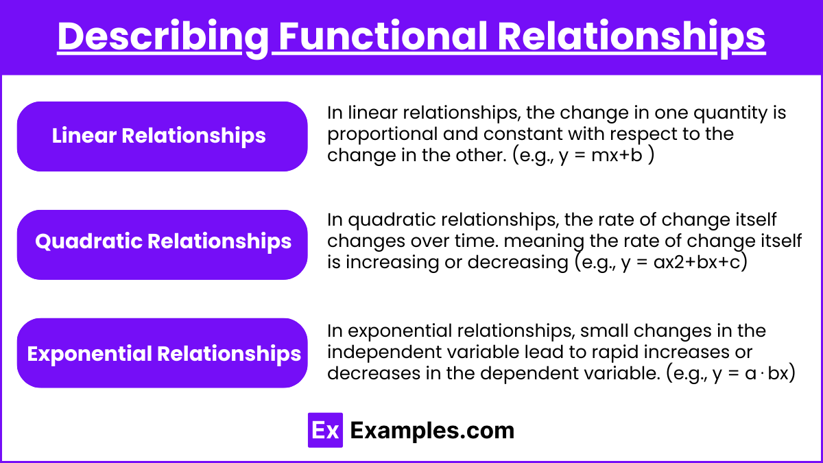
Linear Relationships: The change is proportional and constant (e.g., y = mx+b). In linear relationships, the change in one quantity is proportional and constant with respect to the change in the other. This is represented by the general form y = mx + b, where m is the slope (rate of change) and bbb is the y-intercept. Linear relationships model situations where the rate of change does not vary.

Quadratic Relationships: The change accelerates, meaning the rate of change itself is increasing or decreasing (e.g., y = ax²+bx+c). In quadratic relationships, the rate of change itself changes over time. The general form is y = ax² + bx + c, where aaa, bbb, and ccc are constants. Here, the change in the dependent variable accelerates (or decelerates), creating a parabolic curve.

Exponential Relationships: Small changes in one quantity lead to rapid increases or decreases in the other (e.g., y = a⋅b^x). In exponential relationships, small changes in the independent variable lead to rapid increases or decreases in the dependent variable. The general form is y = a . b^x, where aaa is the initial value, and bbb is the base representing the rate of growth or decay.

Comparing Different Types of Growth

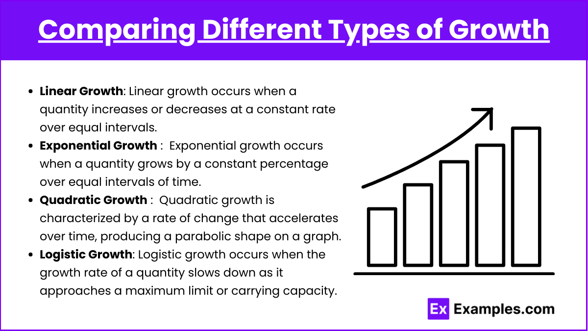
• Linear Growth: A constant rate of increase or decrease, represented by a straight line. Linear growth occurs when a quantity increases or decreases at a constant rate over equal intervals. This type of growth is represented by a straight line on a graph.
• Exponential Growth: Rapid increase or decrease where the rate itself grows over time, often represented by curves that get steeper or shallower. Exponential growth occurs when a quantity grows by a constant percentage (or factor) over equal intervals of time.
• Quadratic Growth: The rate of change increases or decreases in a parabolic shape.Quadratic growth is characterized by a rate of change that accelerates (increases or decreases) over time, producing a parabolic shape on a graph.
• Logistic Growth: Logistic growth occurs when the growth rate of a quantity slows down as it approaches a maximum limit or carrying capacity. This is common in systems where resources are limited.

Applications in Real Life

• Population Growth: In biology, population growth can be modeled using exponential functions, where the population size changes based on factors such as time and resource availability. As resources diminish, the rate of growth can change, leading to logistic growth curves.
• Medicine Dosage and Decay: In pharmacology, the concentration of a drug in the bloodstream decreases exponentially over time. Understanding the rate of decay helps medical professionals determine the appropriate intervals for administering doses to maintain the desired therapeutic levels.
• Weather Patterns: In meteorology, temperature changes with respect to time and geographic location. Understanding how these changes occur helps predict weather patterns, such as how quickly temperatures rise or fall throughout the day, and how atmospheric pressure influences wind speed and direction.
• Electricity Consumption: In electrical engineering, the consumption of electricity changes with respect to time and usage patterns. Monitoring these changes helps utility companies manage energy supply, optimize efficiency, and predict peak usage periods to prevent overloads and outages.

Examples

Example 1: Linear Relationship between Distance and Time

Consider a car moving at a constant speed of 60 miles per hour. In this case, the distance traveled by the car is directly proportional to the time spent driving. For every additional hour the car drives, the distance increases by 60 miles. This constant rate of change illustrates a linear relationship where the slope represents the speed of the car.

Example 2: Exponential Growth in Population

Suppose a town’s population grows at a rate of 5% per year. The population in any given year depends on the population from the previous year, with a 5% increase. This exponential growth means that as time passes, the population increases at an accelerating rate, leading to a steeper increase in later years compared to the early ones. The quantity of population changes with respect to time in a non-linear fashion.

Example 3: Quadratic Relationship in Projectile Motion

When a ball is thrown upwards, its height depends on time and follows a quadratic relationship. Initially, the height increases as the ball ascends, but the rate of increase slows down due to gravity. After reaching its peak height, the ball starts descending, and the height decreases at an accelerating rate. The rate of change of height with respect to time is not constant but varies in a parabolic shape.

Example 4: Temperature and Altitude Relationship

In atmospheric science, the temperature often decreases with increasing altitude. For every 1000 meters in altitude gained, the temperature drops by approximately 6.5 degrees Celsius. This linear relationship between altitude and temperature change illustrates a direct but inverse correlation, where the increase in one quantity (altitude) leads to a decrease in another (temperature).

Example 5: Interest Accumulation in a Bank Account

Consider an account earning compound interest at an annual rate of 4%. The amount of interest earned depends on both the initial principal and the interest accumulated over time. Each year, the interest is calculated on the new total, leading to an exponential increase in the account balance. This example describes how the quantity of money changes with respect to time, with a non-linear and increasing rate of change.

Multiple Choice Questions

Question 1

Which of the following best describes the rate of change in a quadratic function?

A) The rate of change is constant.
B) The rate of change increases or decreases linearly.
C) The rate of change accelerates, meaning it increases or decreases at a non-constant rate.
D) The rate of change decreases exponentially.

Answer: C) The rate of change accelerates, meaning it increases or decreases at a non-constant rate.

Explanation: In a quadratic function (e.g., y = ax² + bx + c), the rate of change is not constant. As you move along the curve, the slope becomes steeper, meaning that the rate at which y changes with respect to x increases or decreases. This behavior is characteristic of quadratic functions, where the rate of change accelerates, unlike linear functions where the rate of change is constant.

Question 2

Given the function y = 5x + 2, which of the following statements is true about the relationship between y and x?

A) y increases by a constant amount as x increases.
B) y decreases exponentially as x increases.
C) y increases quadratically as x increases.
D) The rate of change of y is variable depending on the value of x.

Answer: A) y increases by a constant amount as x increases.

Explanation:
The given function y = 5x + 2 is a linear function, which means that y changes at a constant rate as x increases. Specifically, for every unit increase in x, y increases by 5 units (the coefficient of x represents the slope or constant rate of change). Thus, the relationship between y and x is linear, and the rate of change is constant.

Question 3

Which of the following best describes the average rate of change between two points (x1 ​, y1​) and (x2 , y2) on a function?

A) The average rate of change is the difference in x-values divided by the difference in y-values.
B) The average rate of change is the difference in y-values divided by the difference in x-values.
C) The average rate of change is the sum of the slopes at the two points.
D) The average rate of change can only be determined for linear functions.

Answer: B) The average rate of change is the difference in y-values divided by the difference in x-values.

Explanation:
The average rate of change between two points (x1​,y1​) and (x2,y2) on a function is calculated as: \(\text{Average Rate of Change} = \frac{y_2 – y_1}{x_2 – x_1} \). This represents how much the output (y-value) changes for a given change in the input (xxx-value) and applies to both linear and non-linear functions. The formula is similar to the concept of slope, but it applies across any interval of a function, not just for straight lines.