
Identifying Assumptions and Limitations of Function Models

In AP Precalculus, identifying assumptions and limitations of function models is essential for understanding how accurately they represent real-world phenomena. Function models, such as linear, quadratic, or exponential, rely on assumptions about behavior, continuity, and domain. These models often simplify complex situations, but their accuracy can diminish when applied outside their intended scope. Recognizing limitations, such as extrapolation risks and non-applicability to real-world complexities, helps students critically evaluate when a model is useful and where adjustments are needed to better reflect reality.
Free AP Precalculus Practice Test
Learning Objectives
For the topic "Identifying Assumptions and Limitations of Function Models" in AP Precalculus, you should focus on understanding how function models represent real-world situations by identifying their domain restrictions, simplifying assumptions, and behavioral expectations. Learn to assess the validity of these models by recognizing where they may fail or oversimplify, particularly when extrapolating outside observed data. Additionally, focus on evaluating the accuracy and applicability of models to complex systems, considering factors like continuity, growth patterns, and how limitations affect real-world predictions.
Assumptions of Function Models
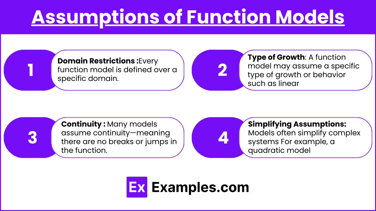
Domain Restrictions: Every function model is defined over a specific domain. This refers to the set of all input values (independent variables) for which the model is valid. Often, real-world scenarios impose natural domain restrictions. For example, a model for population growth may assume that the independent variable (time) cannot be negative.
Type of Growth/Behavior: A function model may assume a specific type of growth or behavior such as linear, quadratic, or exponential. For instance, a linear model assumes constant rates of change, which might not hold for complex real-world phenomena like population growth or decay over time.
Continuity: Many models assume continuity—meaning there are no breaks or jumps in the function. This assumption may not always apply in real-world scenarios where sudden changes can occur.
Simplifying Assumptions: Models often simplify complex systems. For example, a quadratic model for the trajectory of a projectile might assume no air resistance, whereas in reality, air resistance would affect the path.
Limitations of Function Models
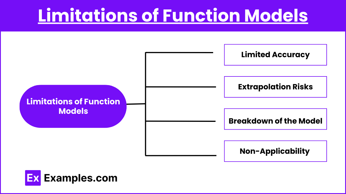
Limited Accuracy: While function models provide useful approximations, they may not always capture all the intricacies of the real-world situation. The further a value deviates from the function’s intended domain, the less accurate the model becomes.
Extrapolation Risks: Predicting behavior outside the known domain (extrapolation) can lead to inaccurate results because the assumptions made by the model may not hold beyond the observed data.
Breakdown of the Model: Certain models only work within specific constraints. For instance, an exponential growth model works well for small populations, but as the population grows, limiting factors (such as food or space) make the model less accurate.
Non-Applicability to Real-World Complexities: Real-world systems are often influenced by multiple variables, whereas function models typically focus on a single or a few factors. This limitation can reduce the model's applicability to more complex systems.
Examples
Example 1: Linear Population Growth Model
A model representing population growth as a linear function assumes a constant rate of growth over time. The assumption is that factors like birth and death rates remain unchanged, which is rarely the case in real-world populations. The limitation of this model is that it cannot account for the slowing of growth as resources become limited or other external factors, making it unreliable over long periods.
Example 2: Quadratic Model for Projectile Motion
When modeling the motion of a projectile, a quadratic function is often used to represent its trajectory. This model assumes that air resistance is negligible and the only force acting on the object is gravity. The limitation here is that in real-world scenarios, air resistance and other forces can significantly alter the path of the projectile, reducing the accuracy of the quadratic model.
Example 3: Exponential Growth of Investment
A function modeling the exponential growth of an investment assumes continuous compounding and a constant interest rate. This model works well for short-term financial projections. However, it has limitations because it does not consider market fluctuations, changes in interest rates, or economic downturns that can affect the growth rate, making long-term predictions unreliable.
Example 4: Rational Function for Supply and Demand
In economics, rational functions are often used to model supply and demand. The assumption is that the relationship between price and quantity supplied or demanded follows a predictable pattern. The limitation of this model is that it cannot account for sudden shifts in consumer behavior, market shocks, or government interventions, which can drastically change the supply-demand relationship.
Example 5: Logistic Growth Model for Population
A logistic function is used to model population growth with a carrying capacity, assuming that as the population grows, resources become scarce, slowing the growth rate. The limitation of this model is that it assumes a fixed carrying capacity and does not account for technological advancements or changes in resource availability that could alter the carrying capacity, making the model less applicable in rapidly changing environments.
Multiple Choice Questions
Question 1
A company models its profit growth using a quadratic function, P(x) = −2x2+10x+500 , where P(x) represents profit in dollars and x is the number of years since the model was created. What assumption is likely made about the company's profit over time?
A. The profit will grow indefinitely.
B. The profit will reach a maximum and then decrease over time.
C. The profit will stay constant over time.
D. The profit will never decrease.
Answer: B. The profit will reach a maximum and then decrease over time.
Explanation: The function is quadratic with a negative coefficient for x2 (i.e., -2). This indicates that the graph is a downward-opening parabola. Quadratic functions with a negative leading coefficient have a maximum point, after which the function decreases. The assumption here is that after a certain point in time, the company’s profit will start to decline.
Question 2
A scientist uses a linear function to model the growth of a plant species, assuming that the height of the plants increases at a constant rate. What is a limitation of using this model for long-term predictions?
A. Linear models do not have a domain.
B. Plants do not always grow at a constant rate indefinitely.
C. Linear functions always overestimate real growth.
D. Linear models are only accurate for small data sets.
Answer: B. Plants do not always grow at a constant rate indefinitely.
Explanation: A linear function assumes constant growth over time, meaning the slope remains the same. However, in reality, plants often experience variable growth rates—faster in early stages and slower as they mature. This is a key limitation, as the assumption of constant growth may not hold for long-term predictions. Over time, environmental factors, resource limitations, and biological constraints affect the plant's growth rate.
Question 3
A logistic function is used to model the population growth of a species in a limited environment. The model assumes that population growth slows as it reaches the environment’s carrying capacity. Which of the following is a limitation of this model?
A. The model assumes no environmental limitations.
B. The model assumes that the population will grow exponentially forever.
C. The model assumes that population growth will stop exactly at the carrying capacity.
D. The model assumes that the population can exceed the carrying capacity.
Answer: C. The model assumes that population growth will stop exactly at the carrying capacity.
Explanation: A logistic growth model assumes that the population will slow down as it nears the carrying capacity, and eventually stop growing once it reaches that capacity. However, real populations may fluctuate around the carrying capacity due to factors like environmental changes, migration, and resource availability. Therefore, assuming the population will stop growing precisely at the carrying capacity is a limitation of this model.