Modeling Aspects of Scenarios Using Polynomial and Rational Functions

In AP Precalculus, modeling real-world scenarios using polynomial and rational functions involves translating complex situations into mathematical expressions. Polynomial functions are ideal for representing continuous processes, such as growth trends or projectile motion, where the degree of the function influences its behavior. Rational functions, on the other hand, model situations involving rates, asymptotes, or undefined points, such as cost efficiency and velocity. Mastering these concepts helps students develop problem-solving skills and provides tools for analyzing diverse, practical problems in areas like physics, economics, and engineering.

Learning Objectives

When studying modeling aspects of scenarios using polynomial and rational functions for AP Precalculus, focus on understanding how these functions describe real-world phenomena. Learn to identify and interpret key features of polynomial functions, such as degree, turning points, and end behavior. For rational functions, focus on asymptotes, holes, and long-term behavior. Practice applying these functions to model scenarios, predict trends, and solve practical problems in fields like physics, economics, and engineering. Graphing and interpreting polynomial and rational functions are also essential skills for mastery.

In AP Precalculus, understanding how to model real-world scenarios using polynomial and rational functions is essential for success. These functions provide frameworks for analyzing trends, predicting outcomes, and explaining behaviors in various contexts such as physics, economics, and biology.

Polynomial Functions

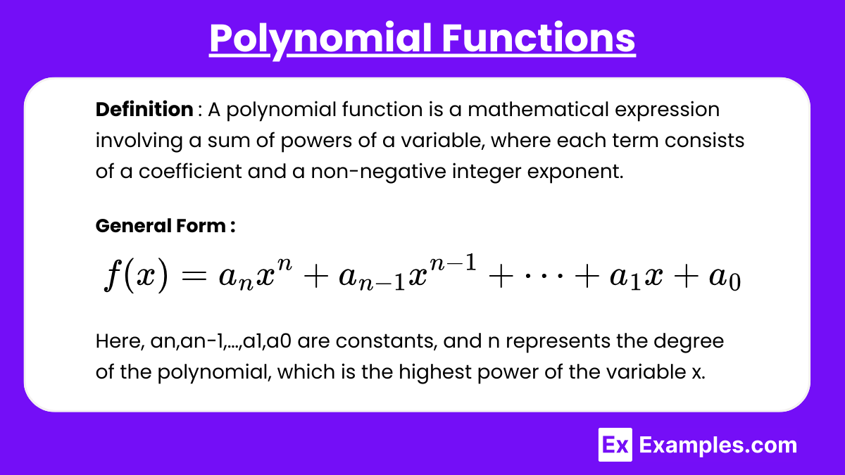
A polynomial function is a mathematical expression involving a sum of powers of a variable, where each term consists of a coefficient and a non-negative integer exponent. The general form of a polynomial function is

\(f(x) = a_n x^n + a_{n-1} x^{n-1} + \dots + a_1 x + a_0 \)

Here, a_n,a_n−1,…,a₁,a₀​ are constants, and n represents the degree of the polynomial, which is the highest power of the variable x. Polynomials are used to represent various real-world phenomena due to their flexibility in modeling smooth and continuous relationships between variables.

• Modeling Real-World Phenomena: Polynomial functions are often used to model situations where the relationship between variables shows a smooth, continuous trend. For example, they can represent the trajectory of a projectile in physics (quadratic functions), population growth, or financial investments over time.
• Identifying Characteristics:
  • Degree of the polynomial influences the general shape of the graph. A higher degree results in more complex behavior (more turning points, inflection points).
  • End behavior describes how the function behaves as x approaches infinity or negative infinity. This is crucial in predicting long-term trends in models like population growth or economic changes.
• Example Scenario:
• In physics, the height h of a ball thrown into the air over time t can be modeled using a quadratic polynomial: \(h(t) = -16t^2 + v_0 t + h_0 \), where v0​ is the initial velocity and h0​ is the initial height.

Rational Functions

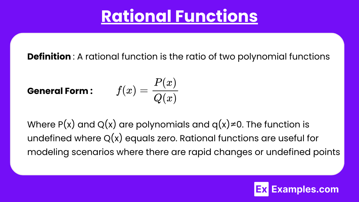
A rational function is the ratio of two polynomial functions: \(f(x) = \frac{P(x)}{Q(x)} \)

Where P(x) and Q(x) are polynomials, and \( q(x) \neq 0 \). The function is undefined where Q(x) equals zero. Rational functions are useful for modeling scenarios where there are rapid changes or undefined points, such as vertical asymptotes, which represent places where the function approaches infinity or breaks down. These functions are commonly applied in fields like physics and economics to describe relationships involving rates of change, cost, or demand.

• Modeling Scenarios: Rational functions model situations where a relationship includes rates of change that can approach infinity or undefined points (such as vertical asymptotes). They are commonly used in physics for modeling speed, force, or work, and in economics to model cost and demand relationships.
• Identifying Key Features:
  • Vertical Asymptotes occur where the denominator Q(x) equals zero. This shows where the model experiences extreme changes or breaks down.
  • Horizontal Asymptotes describe the end behavior as x approaches infinity, indicating a long-term limit or steady-state in a system.
  • Holes in the graph occur where both the numerator and denominator share a common factor.
• Example Scenario: In business, the cost per item C(x) for producing x units of a product might be modeled as: \(C(x) = \frac{100x + 5000}{x} \)
• ​This represents fixed costs ($5000) spread over an increasing number of units x, with a diminishing marginal cost as x grows.

Examples

Example 1. Projectile Motion (Quadratic Polynomial)

When an object is thrown into the air, its height h(t)h(t)h(t) over time ttt can be modeled using a quadratic function. For instance, the equation \( h(t) = -16t^2 + v_0 t + h_0 \) models the height of the object, where v₀​ is the initial velocity and h₀​ is the initial height. This function allows us to predict the time it takes for the object to hit the ground and the maximum height it reaches.

Example 2. Revenue and Profit Maximization (Cubic Polynomial)

In business, companies often model their total revenue or profit as a cubic polynomial function of the number of units sold. For example, if a company finds that its profit can be modeled by \( P(x) = -2x^3 + 15x^2 – 10x + 500 \), where x is the number of units sold, the function helps to identify the point at which profit is maximized by analyzing the turning points of the polynomial.

Example 3. Cost Per Unit (Rational Function)

In manufacturing, the cost per unit of production is often modeled using a rational function. For example, \( C(x) = \frac{100x + 5000}{x} \)​ models the cost per unit of producing xxx units of a product, where $5000 represents the fixed cost, and $100 represents the variable cost per unit. This function shows that as the number of units produced increases, the cost per unit decreases.

Example 4. Population Growth (Polynomial Function)

In ecology, polynomial functions are used to model population growth over time. For instance, the population of a certain species may be modeled as \( P(t) = 2t^3 – 10t^2 + 50t + 100 \), where t represents time in years. This model can help predict future population trends, determine the year when the population reaches its maximum, or when it starts to decline.

Example 5. Drug Concentration in the Blood (Rational Function)

In pharmacokinetics, the concentration of a drug in the bloodstream over time can be modeled using a rational function. For example, \( C(t) = \frac{a}{t+b} \)​, where aaa and bbb are constants, and t represents time. This model helps predict how long the drug will remain in the system and when the concentration will be highest, aiding in proper dosage planning.

Multiple Choice Questions

Question 1

A company’s profit P(x) in dollars, where x is the number of units sold, is modeled by the polynomial function P(x) = −2x²+20x−50. What is the number of units x that maximizes the company’s profit?

A) 5
B) 10
C) 20
D) 50

Answer: A) 5

Explanation: This is a quadratic function P(x) = −2x²+20x−50, which is a downward-facing parabola (because the coefficient of x² is negative). The maximum value occurs at the vertex. The formula for finding the vertex of a parabola ax²+bx+c is given by: \(x = -\frac{b}{2a} \)

Substitute a=−2 and b=20 into the formula: \(x = -\frac{20}{2(-2)} = 5 \)

Thus, the maximum profit occurs when 5 units are sold.

Question 2

A rational function is used to model the concentration of a drug in the bloodstream over time, given by \(C(t) = \frac{a}{t + b}\)​, where a and b are constants and t is time. Which of the following statements about the behavior of the function is correct?

A) The concentration will continue to increase as t increases.
B) The concentration approaches zero as t increases.
C) The concentration will reach a maximum and then decrease.
D) The concentration is constant over time.

Answer: B) The concentration approaches zero as t increases.

Explanation: This function \(C(t) = \frac{a}{t + b}\)​ is a rational function, where t+b in the denominator causes the function to decrease as t increases. As t becomes very large, the value of C(t) approaches zero because the denominator t+b grows much larger than the numerator a, causing the overall value of the function to shrink. Therefore, the concentration of the drug decreases over time and approaches zero.

Question 3

Which of the following functions is best suited for modeling a real-world scenario where there is a fixed cost and a variable cost that decreases as the number of units produced increases?

A) C(x) = 100x+5000
B) \( C(x) = \frac{100x + 5000}{x} \)
C) C(x) = −5x²+200x
D) \( C(x) = \frac{5000}{x} \)

Answer: B) \( C(x) = \frac{100x + 5000}{x} \)

Explanation: The function that models a fixed cost and a variable cost that decreases as production increases is best represented by a rational function. In this case, \( C(x) = \frac{100x + 5000}{x} \)​ includes a fixed cost of $5000 and a variable cost per unit of $100. As the number of units produced (x) increases, the cost per unit decreases because the fixed cost is spread over more units.