Home
AP Precalculus
Modeling Data Sets With Exponential Functions

Modeling Data Sets With Exponential Functions

Modeling data sets with exponential functions is a key concept in AP Precalculus, often used to describe real-world phenomena such as population growth, radioactive decay, and compound interest. An exponential function takes the form 𝑦 = 𝑎𝑏^𝑥, where 𝑎 is the initial value, 𝑏 is the growth or decay factor, and 𝑥 is the independent variable. Recognizing exponential patterns in data allows for accurate modeling, prediction, and interpretation of scenarios that involve rapid changes or steady percentage increases or decreases over time.

Free AP Precalculus Practice Test

Learning Objectives

For the topic “Modeling Data Sets With Exponential Functions” in AP Precalculus, you should learn to identify exponential patterns in real-world data, distinguish between exponential growth and decay, and accurately fit data to exponential models. You will develop skills to interpret the meaning of the initial value and growth/decay rate, apply logarithmic transformations to linearize exponential data, and validate the accuracy of your models by analyzing their fit. Understanding applications like population growth, radioactive decay, and finance will also be crucial.

In AP Precalculus, you are expected to model data sets using exponential functions. This process involves identifying relationships in data where the rate of change is proportional to the value of the function itself. This is common in situations involving growth or decay, such as population growth, radioactive decay, or compound interest.Key Concepts:

Exponential Function Form

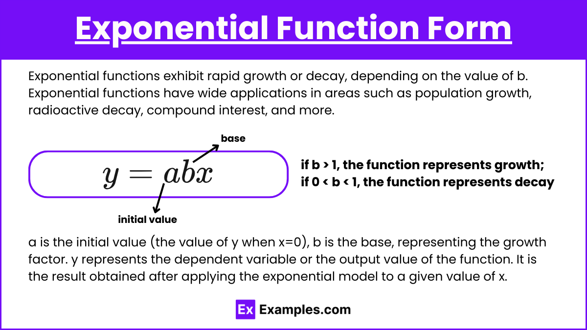
Exponential functions exhibit rapid growth or decay, depending on the value of b. Exponential functions have wide applications in areas such as population growth, radioactive decay, compound interest, and more. They are characterized by their rapid growth or decay, depending on the value of b. The graph of an exponential function exhibits a curved shape, and it never touches the x-axis (horizontal asymptote), approaching it as x→−∞ but never reaching zero.

An exponential function is of the form y = ab^x,

where:

a is the initial value (the value of y when x=0),
b is the base, representing the growth factor (if b > 1, the function represents growth; if 0 < b < 1, the function represents decay),
y represents the dependent variable or the output value of the function. It is the result obtained after applying the exponential model to a given value of x.
x is the independent variable (often representing time in applications).

Exponential Growth and Decay

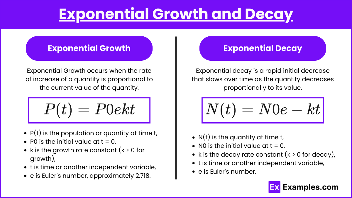
Exponential Growth occurs when the rate of increase of a quantity is proportional to the current value of the quantity, leading to a rapid increase as time progresses. This type of growth is characterized by a constant percentage increase over equal time intervals, which leads to the function becoming steeper and increasing more rapidly as x (often time) increases. The general formula for exponential growth is :

P(t) = P₀e^kt

where:

P(t) is the population or quantity at time t,
P₀ is the initial value at t = 0,
k is the growth rate constant (k > 0 for growth),
t is time or another independent variable,
e is Euler’s number, approximately 2.718.

Exponential Decay occurs when the rate of decrease of a quantity is proportional to the current value of the quantity, leading to a rapid decrease initially that slows down over time. This type of decay is characterized by a constant percentage decrease over equal time intervals, which leads to the function becoming flatter and approaching zero as x increases. The general formula for exponential decay is:

N(t) = N₀e^−kt

where:

N(t) is the quantity at time t,
N₀ is the initial value at t = 0,
k is the decay rate constant (k > 0 for decay),
t is time or another independent variable,
e is Euler’s number.

Logarithmic Transformation

To linearize exponential data, you can apply logarithms to both sides of the equation. This transforms the exponential relationship into a linear one:

If y = ab^x, then logy = loga + xlogb.

This allows you to fit a linear model to logarithmic data, making it easier to analyze and interpret.

Steps for Modeling with Exponential Functions

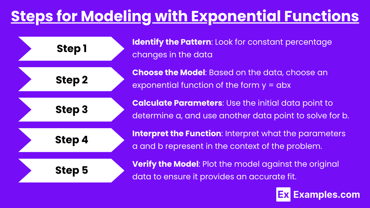
Step 1: Identify the Pattern: Look for constant percentage changes in the data, which is a hallmark of exponential growth or decay.
Step 2: Choose the Model: Based on the data, choose an exponential function of the form y = ab^x.
Step 3: Calculate Parameters: Use the initial data point to determine a, and use another data point to solve for b.
Step 4: Interpret the Function: Once the model is established, interpret what the parameters a and b represent in the context of the problem.
Step 5: Verify the Model: Plot the model against the original data to ensure it provides an accurate fit.

Applications

Finance: Modeling compound interest using $A(t) = P \left( 1 + \frac{r}{n} \right)^{nt}$, where A(t) is the amount after time t, P is the principal, r is the annual interest rate, and n is the number of times the interest is compounded per year.
Population Dynamics: Modeling populations that grow at a constant percentage rate using P(t) = P₀e^kt.
Physics and Chemistry: Modeling radioactive decay or cooling processes where quantities decrease over time according to exponential decay laws.

Examples

Example 1: Population Growth

Suppose the population of a city is growing at a rate of 5% per year. The initial population is 100,000. You can model this growth using the exponential function P(t) = 100,000 × (1.05)^t, where t is the number of years. As t increases, the population grows exponentially. For instance, after 10 years, the population will be approximately 162,889. This exponential model helps predict future population sizes based on current growth trends.

Example 2: Radioactive Decay

A radioactive substance decays at a rate of 3% per hour. The initial amount is 500 grams. The exponential decay function is N(t) = 500 × (0.97)^t, where t represents time in hours. After 5 hours, the remaining quantity of the substance will be around 427.68 grams. This model is useful in predicting the amount of radioactive material left after a certain period and is widely used in nuclear physics and chemistry.

Example 3: Compound Interest

An individual invests $1,000 in a savings account with an annual interest rate of 4%, compounded quarterly. The amount of money after t years is modeled by $A(t) = 1000 \times \left( 1 + \frac{0.04}{4} \right)^{4t}\ $. For example, after 5 years, the balance will be approximately $1,221.39. This exponential model is crucial in finance for understanding how investments grow over time with compound interest.

Example 4: Bacterial Growth

A bacterial colony grows at a constant rate, doubling in size every 3 hours. If the initial population is 200 bacteria, the population after t hours is modeled by P(t) = 200 × 2 ^t/3. For example, after 9 hours, the population will be approximately 1,600 bacteria. This exponential growth model is essential in biology for predicting the growth of bacterial colonies under controlled conditions.

Example 5: Cooling of an Object

According to Newton’s Law of Cooling, the temperature of a hot object decreases exponentially over time as it approaches room temperature. If a cup of coffee initially at 90°C is left in a room where the temperature is 20°C, the temperature of the coffee T(t) after t minutes can be modeled as T(t) = 20+(90−20) × e^−kt, where k is a constant. This model helps predict how quickly the coffee cools down to room temperature.

Multiple Choice Questions

Question 1

A certain bacteria population doubles every 3 hours. If the initial population is 500 bacteria, which of the following equations best models the population size P(t), in bacteria, after t hours?

A) $ P(t) = 500(2^t) $
B) $ P(t) = 500(2^{t/3}) $
C) $ P(t) = 500e^{0.231t} $
D) $ P(t) = 500 + 2t $

Answer: B

Explanation: The bacteria population is growing exponentially because it doubles at a constant rate. The doubling time is every 3 hours, so the base of the exponential function is 2, but the exponent must account for the time in hours divided by the doubling time:

The equation is of the form $ P(t) = P_0b^{t/T} $, where P0 is the initial population, b=2 (since the population doubles), and T=3 (because doubling occurs every 3 hours).
Therefore, the correct model is $ P(t) = 500(2^{t/3}) $, which is option B.

Question 2

Which of the following best describes the end behavior of the exponential function $ P(t) = 300(0.85^t) $, where t represents time in years?

A) The population will grow without bound as t increases.
B) The population will decay to 300 as t increases.
C) The population will approach zero as t increases.
D) The population will increase by 85% each year.

Answer: C

Explanation: The given function is of the form $ P(t) = ab^t $, where a=300 and b=0.85. Since 0 < b < 1, this represents an exponential decay function. As t increases, the value of 0.85t gets smaller and smaller, approaching zero. Thus, the population approaches zero over time, which makes option C the correct answer.

Question 3

A certain investment grows at an annual rate of 6%. If the initial investment was $1,000, which equation represents the value V(t) of the investment after t years?

A) V(t) = 1000(1.06)^t
B) V(t) = 1000(0.06^t)
C) V(t) = 1000(1+0.06t)
D) V(t) = 1000(1.6)^t

Answer: A

Explanation: The investment is growing at a constant percentage rate (6% per year), which indicates exponential growth. The general form for exponential growth is V(t) = P(1+r)^t, where P is the initial value, and r is the growth rate. In this case:

P=1000,
r=0.06 (6% annual growth rate).

Thus, the correct equation is V(t) = 1000(1.06)^t, making option A the correct answer.