Modeling Scenarios with Logarithmic Functions

Logarithmic functions are crucial in modeling scenarios involving processes that grow rapidly but slow down over time. Commonly seen in real-world applications like population growth, sound intensity, and the Richter scale for earthquakes, logarithmic functions provide a way to understand exponential relationships. These models are useful in cases where the input grows exponentially while the output changes more gradually. Understanding how to apply logarithmic functions is essential for interpreting data and solving complex problems in AP Precalculus.

Learning Objectives

In studying “Modeling Scenarios with Logarithmic Functions” for AP Precalculus, you should aim to understand how logarithmic functions are applied to real-world scenarios, such as population growth, sound intensity, and earthquake magnitude. You should learn how to graph logarithmic functions, analyze transformations (shifts, stretches, reflections), and interpret their behavior, including asymptotes and domain restrictions. Additionally, you should be able to identify when logarithmic models are appropriate, apply them to given data sets, and solve problems involving logarithmic equations in various practical contexts.

Logarithmic Function Basics

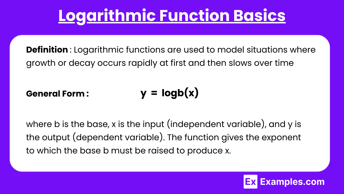
Logarithmic functions are used to model situations where growth or decay occurs rapidly at first and then slows over time. Common real-world scenarios that involve logarithmic functions include sound intensity, pH levels, and population growth that approaches a limiting value. A logarithmic function is the inverse of an exponential function. It has the form:

y = log_b​(x)

where b is the base, x is the input (independent variable), and y is the output (dependent variable). The function gives the exponent to which the base b must be raised to produce x.

Real-World Applications of Logarithmic Functions

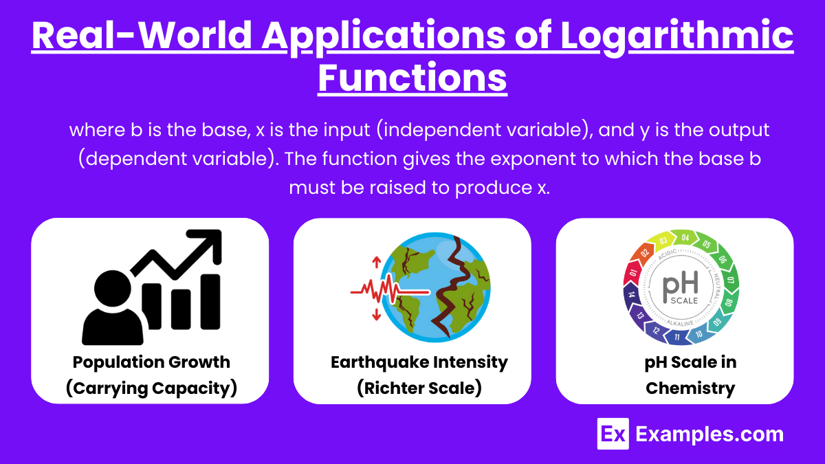
Logarithmic functions are used to model scenarios where growth or decay occurs at a decreasing rate. Common real-world applications include measuring earthquake intensity with the Richter scale, analyzing sound intensity in decibels, calculating population growth, and determining the half-life of radioactive materials. These functions help simplify complex multiplicative relationships.Logarithmic models are commonly used in:

• Population Growth (Carrying Capacity): As populations grow, they often approach a maximum capacity due to limited resources. The growth slows down as the population size approaches the carrying capacity, and this phenomenon can be modeled using logarithmic functions.
• Earthquake Intensity (Richter Scale): The magnitude of an earthquake is measured on a logarithmic scale where each whole number increase corresponds to a tenfold increase in measured amplitude.
• pH Scale in Chemistry: The pH scale, used to measure the acidity or basicity of solutions, is a logarithmic scale. Each unit change represents a tenfold change in hydrogen ion concentration.

Modeling Process

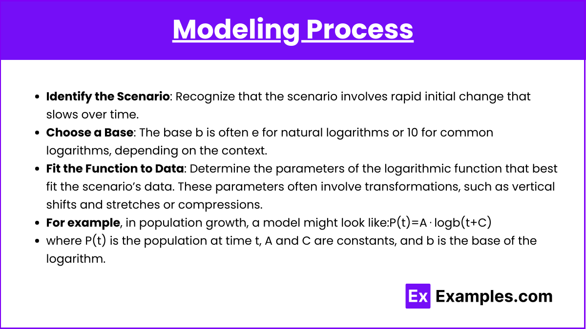
When modeling real-world scenarios with logarithmic functions, the following steps are typically followed:

• Identify the Scenario: Recognize that the scenario involves rapid initial change that slows over time.
• Choose a Base: The base b is often e for natural logarithms or 10 for common logarithms, depending on the context.
• Fit the Function to Data: Determine the parameters of the logarithmic function that best fit the scenario’s data. These parameters often involve transformations, such as vertical shifts and stretches or compressions.

For example, in population growth, a model might look like:P(t)=A⋅logb​(t+C)

where P(t) is the population at time t, A and C are constants, and b is the base of the logarithm.

Graphing Logarithmic Functions

Graphically, logarithmic functions have a vertical asymptote (usually at x=0) and increase slowly as x increases. The function approaches infinity as x increases but does so at a decreasing rate. Understanding the behavior of the graph is important when interpreting real-world data modeled by logarithmic functions.

Transformations

When modeling with logarithmic functions, transformations are essential to fit the model to the data. Common transformations include:

• Vertical Shifts (adding a constant to the function)
• Horizontal Shifts (adding or subtracting from the input variable)
• Reflections (multiplying the function by -1 for reflection over the x-axis)
• Stretches and Compressions (multiplying the function by a constant).

Examples

Example 1: Earthquake Magnitude (Richter Scale)

The magnitude of an earthquake, as measured on the Richter scale, is a logarithmic function of the amplitude of seismic waves. The equation \( M = \log\left(\frac{A}{A_0}\right) \), where M is the earthquake’s magnitude, A is the amplitude of the seismic waves, and A₀​ is a reference amplitude, demonstrates how small increases in the logarithmic value reflect large changes in energy release.

Example 2: pH Levels in Chemistry

The pH of a solution is modeled logarithmically as \( \text{pH} = -\log [H^+] \), where [H+] is the concentration of hydrogen ions. This logarithmic relationship helps chemists understand the acidity or basicity of a solution. Small changes in pH represent significant changes in hydrogen ion concentration, making logarithmic functions crucial in pH calculations.

Example 3: Sound Intensity (Decibels)

The loudness of sound in decibels is modeled using the logarithmic equation \( L = 10 \log\left(\frac{I}{I_0}\right) \), where L is the loudness in decibels, I is the intensity of the sound, and I0​ is the reference intensity. This equation shows that a small increase in decibel level represents a much larger increase in actual sound intensity.

Example 4: Population Growth with Resource Limits

In ecological studies, populations that initially grow rapidly but slow down as they approach environmental carrying capacity can be modeled logarithmically. The function P(t) = klog(t) + C shows how population P increases over time t but eventually plateaus, reflecting the limitations of available resources like food and space.

Example 5: Compound Interest in Economics

In finance, the time required to reach a specific investment goal under compound interest can be modeled with logarithmic functions. The equation \( t = \frac{\log\left(\frac{A}{P}\right)}{n \log(1 + r)} \)​ relates the time t to the principal P, final amount A, interest rate r, and number of periods n. This logarithmic relationship helps in calculating the time needed for an investment to grow to a target value.

Multiple Choice Questions

Question 1

Which of the following scenarios can be best modeled by a logarithmic function?

A. The distance traveled by a car over time at a constant speed.
B. The growth of a bacterial population in an ideal environment.
C. The increase in sound intensity as the loudness in decibels increases.
D. The decay of a radioactive substance over time.

Answer: C. The increase in sound intensity as the loudness in decibels increases.

Explanation: The loudness of sound in decibels is modeled by a logarithmic function because the increase in decibel level corresponds to a proportional increase in sound intensity, but not linearly. Decibel level grows logarithmically relative to sound intensity, reflecting how humans perceive changes in loudness. Other scenarios such as constant speed travel (A) and exponential growth or decay (B and D) are better modeled by linear or exponential functions, not logarithmic ones.

Question 2

The pH of a solution is given by pH=−log[H+], where [H+] represents the concentration of hydrogen ions. If the concentration of hydrogen ions in a solution decreases by a factor of 10, what happens to the pH?

A. The pH decreases by 1 unit.
B. The pH increases by 1 unit.
C. The pH decreases by 10 units.
D. The pH remains the same.

Answer: B. The pH increases by 1 unit.

Explanation: The relationship between pH and hydrogen ion concentration is logarithmic. Since pH is the negative logarithm of the hydrogen ion concentration, decreasing the concentration by a factor of 10 means the value inside the logarithmic expression becomes 10 times smaller. The logarithmic function log(10) = 1, so the pH increases by 1 unit for every tenfold decrease in [H+].

Question 3

Which of the following equations represents a logarithmic model that could be used to describe the growth of a population that initially grows rapidly but slows down over time?

A. P(t) = 100e^0.05t
B. P(t) = 500−100t
C. P(t) = 100log(t)+200
D. P(t) = 100−50e^−0.1t

Answer: C. P(t) = 100log(t)+200

Explanation: The equation P(t)=100log(t)+200 is a logarithmic function that models a situation where population growth is rapid initially but slows down over time. The logarithmic function reflects this type of growth behavior because it increases quickly for small values of t and then levels off as t becomes larger. The other options represent exponential growth (A), linear change (B), or exponential decay (D), which do not fit the scenario of slowing growth.