Calculating and Interpreting Statistics

In AP Statistics, calculating and interpreting statistics involves understanding and using graphs to visually represent data. Graphs, such as histograms, boxplots, scatter plots, and bar charts, help summarize data distributions, identify patterns, and compare different datasets. Mastering these graphical representations enables students to effectively communicate statistical findings, interpret measures of central tendency and spread, and make informed decisions based on data analysis. These skills are essential for success in the AP Statistics exam.

Learning Objectives

By studying calculating and interpreting statistics, you will learn to create and interpret various graphs such as histograms, boxplots, scatter plots, and bar charts. You will understand how to summarize data distributions, identify patterns, and compare datasets visually. These skills will help you effectively communicate statistical findings and interpret measures of central tendency and spread. Mastering these concepts will enhance your data analysis abilities, preparing you for success in the AP Statistics exam.

Descriptive Statistics

Measures of Central Tendency

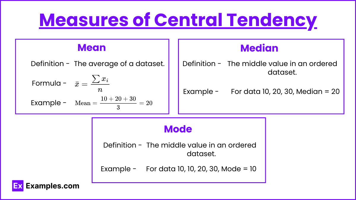
• Mean: The average of a dataset.
  • Formula: \[\bar{x} = \frac{\sum x_i}{n}\]
  • Example: \[\text{Mean} = \frac{10 + 20 + 30}{3} = 20\]
• Median: The middle value in an ordered dataset.
  • Example: For data 10, 20, 30, Median = 20
• Mode: The most frequently occurring value in a dataset.
  • Example: For data 10, 10, 20, 30, Mode = 10

Measures of Spread

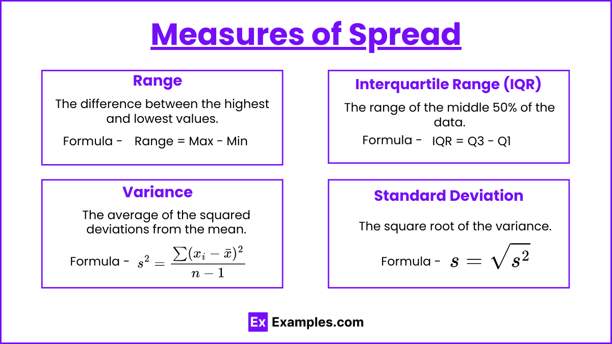
• Range: The difference between the highest and lowest values.
  • Formula: Range = Max – Min
  • Example: For data 10, 20, 30, Range = 30 – 10 = 20
• Interquartile Range (IQR): The range of the middle 50% of the data.
  • Formula: IQR = Q3 – Q1
  • Example: For data 10, 20, 30, 40, 50, Q1 = 20, Q3 = 40, IQR = 40 – 20 = 20
• Variance: The average of the squared deviations from the mean.
  • Formula: \[s^2 = \frac{\sum (x_i – \bar{x})^2}{n – 1}\]
  • Example: For data 10, 20, 30, Mean = 20, Variance = \[\text{Variance} = \frac{(10-20)^2 + (20-20)^2 + (30-20)^2}{2} = \frac{100}{2} = 50\]
• Standard Deviation: The square root of the variance.
  • Formula: s = \[\sqrt{s^2}\]
  • Example: For data 10, 20, 30, Variance = 100, \[\text{Standard Deviation} = \sqrt{50} \approx 7.07\]

Inferential Statistics

Confidence Intervals

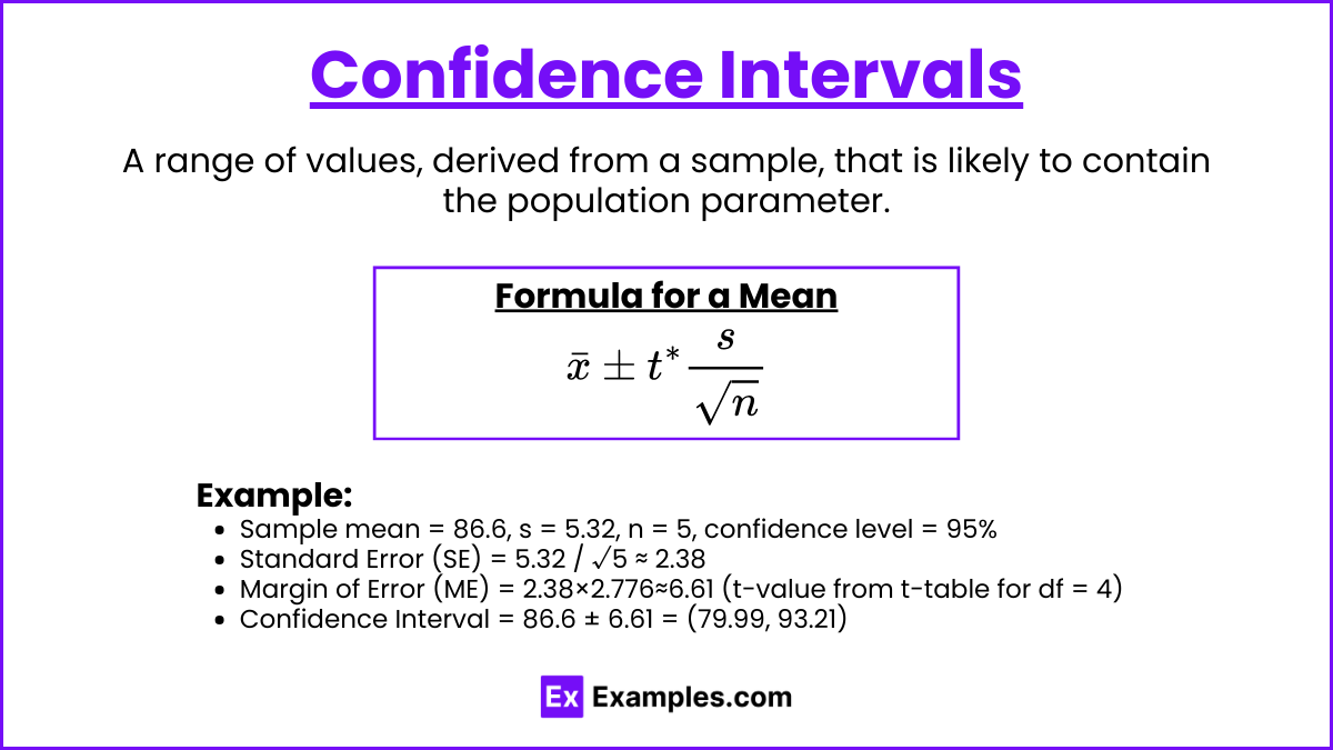
• Definition: A range of values, derived from a sample, that is likely to contain the population parameter.
• Formula for a Mean:\[ \bar{x} \pm t^× \frac{s}{\sqrt{n}}\]
• Example: Sample mean = 86.6, s = 5.32, n = 5, confidence level = 95%
  • Standard Error (SE) = 5.32 / √5 ≈ 2.38
  • Margin of Error (ME) = 2.38×2.776≈6.61 (t-value from t-table for df = 4)
  • Confidence Interval = 86.6 ± 6.61 = (79.99, 93.21)

Hypothesis Testing

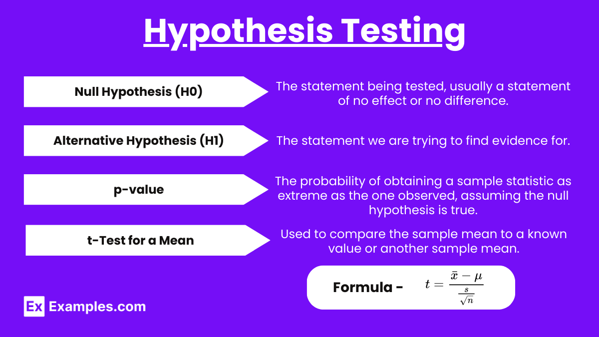
• Null Hypothesis (H0): The statement being tested, usually a statement of no effect or no difference.
• Alternative Hypothesis (H1): The statement we are trying to find evidence for.
• p-value: The probability of obtaining a sample statistic as extreme as the one observed, assuming the null hypothesis is true.
• t-Test for a Mean: Used to compare the sample mean to a known value or another sample mean.
  • Formula: \[t = \frac{\bar{x} – \mu}{\frac{s}{\sqrt{n}}}\]
  • Example: Sample mean = 86.6, population mean = 90, s = 5.32, n = 5
    • t = (86.6 – 90) / (5.32 / √5) ≈ -1.63

Examples

Example 1: Calculating the Mean

• Data: Test scores: 85, 90, 78, 92, 88
• Calculation: Mean = (85 + 90 + 78 + 92 + 88) / 5 = 86.6

Example 2: Calculating the Median

• Data: Test scores: 85, 90, 78, 92, 88
• Calculation: Ordered data: 78, 85, 88, 90, 92. Median = 88

Example 3: Calculating the Standard Deviation

• Data: Test scores: 85, 90, 78, 92, 88
• Calculation:
  • Mean = 86.6
  • Variance = [(85-86.6)² + (90-86.6)² + (78-86.6)² + (92-86.6)² + (88-86.6)²] / 5 = 28.24
  • Standard Deviation = √28.24 ≈ 5.32

Example 4: Confidence Interval for a Mean

• Data: Sample mean = 86.6, standard deviation = 5.32, n = 5, confidence level = 95%
• Calculation:
  • Standard Error (SE) = 5.32 / √5 ≈ 2.38
  • Margin of Error (ME) = 2.38 × 2.776 ≈ 6.61 (t-value from t-table for df = 4)
  • Confidence Interval = 86.6 ± 6.61 = (79.99, 93.21)

Example 5: Hypothesis Testing (t-Test)

• Data: Sample mean = 86.6, population mean = 90, standard deviation = 5.32, n = 5
• Hypothesis:
  • Null Hypothesis (H0): μ = 90
  • Alternative Hypothesis (H1): μ ≠ 90
• Calculation:
  • t = (86.6 – 90) / (5.32 / √5) ≈ -1.63
  • Compare t to critical t-value from t-table (df = 4). If t is outside the range, reject H0.

Multiple Choice Questions

Question 1: What is the median of the dataset: 12, 15, 14, 18, 17?

A. 12
B. 15
C. 14
D. 17

Answer: C. 14

Explanation: When the data is ordered (12, 14, 15, 17, 18), the median is the middle value, which is 14.

Question 2: What does a standard deviation measure?

A. The average value of the dataset
B. The range of the dataset
C. The average distance from the mean
D. The most frequently occurring value

Answer: C. The average distance from the mean

Explanation: The standard deviation measures the average distance of each data point from the mean of the dataset.

Question 3: In hypothesis testing, what does a p-value represent?

A. The probability of the null hypothesis being true
B. The probability of obtaining the observed sample results if the null hypothesis is true
C. The average value of the sample
D. The standard deviation of the population

Answer: B. The probability of obtaining the observed sample results if the null hypothesis is true

Explanation: The p-value represents the probability of obtaining a sample statistic as extreme as the one observed, assuming the null hypothesis is true.