
Confidence Intervals and Tests For the Difference of 2 Population Means

In AP Statistics, confidence intervals and hypothesis tests for the difference of two population means are essential tools for comparing two groups based on sample data. These methods allow students to determine whether observed differences in sample means reflect actual differences between the populations or if they could be attributed to random variation. By constructing confidence intervals, students can estimate a range of plausible values for the difference between two population means, providing a level of certainty about this difference. Hypothesis testing, on the other hand, enables students to make data-driven decisions about whether there is statistically significant evidence to support claims about population means. Together, these techniques are fundamental for analyzing and interpreting differences between two groups in various real-world contexts.
Learning Objective
In this lesson on confidence intervals and tests for the difference of two population means, you will be introduced to the methods for estimating the difference between two population means using sample data. You will be guided through the process of constructing confidence intervals and conducting hypothesis tests to determine if observed differences are statistically significant. Additionally, you will be expected to understand the assumptions underlying these methods and learn to interpret results in the context of real-world scenarios.
Definition:
A confidence interval provides a range of plausible values for the difference between two population means,  , based on sample data. The interval is constructed so that, with a specified level of confidence (usually 95%), it contains the true difference between the population means.
Formulas
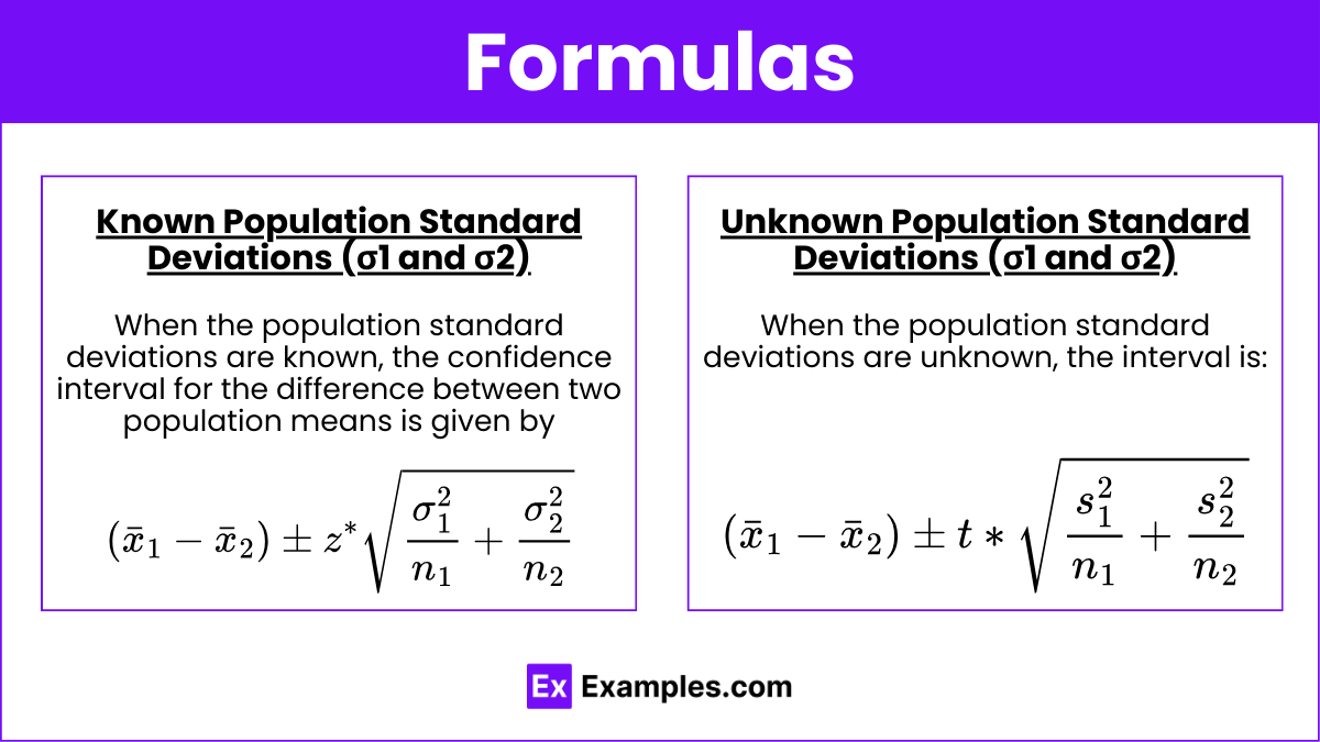
There are two cases to consider when constructing confidence intervals:
a) Known Population Standard Deviations (σ1 and σ2)
When the population standard deviations are known, the confidence interval for the difference between two population means is given by:
 and
and  are the sample means.
 and
and  are the sample sizes.
- σ1 and σ2 are the population standard deviations.
- z* is the critical value from the standard normal distribution for the desired confidence level.
b) Unknown Population Standard Deviations (σ1 and σ2)
When the population standard deviations are unknown, the interval is:

- s₁ and s₂ are the sample standard deviations.
- t* is the critical value from the t-distribution with degrees of freedom calculated using the following approximation:

Interpretation:
If a 95% confidence interval for μ1−μ2 is [−2,5], we can say that we are 95% confident that the true difference between the population means lies between -2 and 5. If 0 is within this interval, it suggests that there may be no significant difference between the two population means.
Hypothesis Tests for the Difference of Two Population Means
Definition:
A hypothesis test allows us to use sample data to evaluate a claim about the difference between two population means.
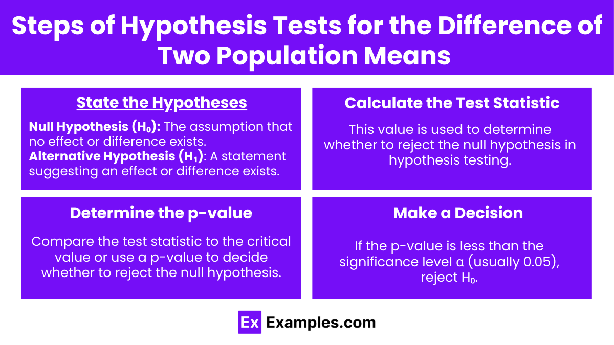
Steps:
- State the Hypotheses:
- Null Hypothesis (H₀): μ1−μ2=0 (There is no difference between the population means).
- Alternative Hypothesis (H₁): μ1−μ2≠0 (Two-tailed test), μ1−μ2>0 (Right-tailed test), or μ1−μ2<0 (Left-tailed test).
- Calculate the Test Statistic:
- For known σ1 and σ2:

- For unknown σ1 and σ2:

where the degrees of freedom are calculated as mentioned earlier. - Determine the p-value:
- Compare the test statistic to the critical value or use a p-value to decide whether to reject the null hypothesis.
- Make a Decision:
- If the p-value is less than the significance level α (usually 0.05), reject H₀.
Example Hypotheses:
- Two-tailed test:

- One-tailed test (right):

- One-tailed test (left):

Assumptions
For both confidence intervals and hypothesis tests, the following assumptions should hold:
- Independent Samples: The two samples should be independent of each other.
- Normality: The population from which the samples are drawn should be approximately normally distributed, especially for small sample sizes.
- Sample Size: For large sample sizes, the Central Limit Theorem ensures that the sampling distribution of the difference in means will be approximately normal even if the populations are not normal.
Examples
Example 1: Confidence Interval with Known σ1 and σ2
Two samples are taken from two different populations. Sample 1 has a mean of 30, a standard deviation of 5, and a sample size of 40. Sample 2 has a mean of 28, a standard deviation of 6, and a sample size of 35. Construct a 95% confidence interval for the difference between the population means.
Solution:![\text{CI} = (30 - 28) \pm 1.96 \sqrt{\frac{5^2}{40} + \frac{6^2}{35}} = 2 \pm 1.96 \times 1.304 \approx 2 \pm 2.55 = [-0.55, 4.55]](https://www.examples.com/wp-content/ql-cache/quicklatex.com-50a5427bad4ab84c2312b7866cd80630_l3.svg "Rendered by QuickLaTeX.com")
Interpretation: We are 95% confident that the true difference between the population means is between -0.55 and 4.55.
Example 2: Hypothesis Test with Unknown σ1 and σ2
Researchers are comparing the mean weights of two different species of birds. They collect a sample of 20 birds from species A, with a sample mean weight of 1.5 kg and a sample standard deviation of 0.2 kg. For species B, they collect 25 birds, with a sample mean weight of 1.3 kg and a sample standard deviation of 0.25 kg. Test the hypothesis at the 0.05 significance level that there is no difference in the mean weights of the two species.
Solution: 
Using a t-table, the critical value for a two-tailed test with  at α=0.05 is 2.024. Since 2.56 > 2.024, we reject H₀.
Conclusion: There is sufficient evidence to conclude that there is a significant difference in the mean weights of the two species.
Example 3: Large Sample Confidence Interval
A company wants to compare the average productivity between two of its plants. They take a random sample of 100 workers from plant A and find an average output of 50 units per day with a standard deviation of 8 units. From plant B, they take a sample of 120 workers and find an average output of 47 units per day with a standard deviation of 7 units. Construct a 90% confidence interval for the difference in average productivity.
Solution: ![\text{CI} = (50 - 47) \pm 1.645 \sqrt{\frac{8^2}{100} + \frac{7^2}{120}} \approx 3 \pm 1.645 \times 1.04 = 3 \pm 1.71 = [1.29, 4.71]](https://www.examples.com/wp-content/ql-cache/quicklatex.com-2c5627c20e0ee8e0a1dbf36cbb2235a2_l3.svg "Rendered by QuickLaTeX.com")
Interpretation: We are 90% confident that the difference in average productivity between the two plants is between 1.29 and 4.71 units per day.
Example 4: One-Tailed Hypothesis Test
A dietician wants to test if a new diet plan has a different effect on weight loss compared to an old plan. She takes a sample of 15 participants from each plan. For the new plan, the mean weight loss is 5 kg with a standard deviation of 1 kg. For the old plan, the mean weight loss is 4.5 kg with a standard deviation of 1.2 kg. Test at the 0.10 significance level whether the new plan leads to greater weight loss.
Solution: 
For a one-tailed test with df=28, the critical value at α=0.10 is 1.311. Since 1.32 > 1.311, we reject H₀.
Conclusion: There is evidence at the 0.10 level that the new plan leads to greater weight loss.
Example 5: Equal Variance Assumption
Suppose the average test scores of two classes are being compared. Class A has 25 students with a mean score of 78 and a standard deviation of 10. Class B has 30 students with a mean score of 82 and a standard deviation of 9. Assuming equal variances, construct a 95% confidence interval for the difference in means.
Solution:

![\text{CI} = (78 - 82) \pm 2.048 \sqrt{90.91 \times \left(\frac{1}{25} + \frac{1}{30}\right)} = -4 \pm 2.048 \times 2.95 \approx [-9.04, 1.04]](https://www.examples.com/wp-content/ql-cache/quicklatex.com-c4d236c686e887fbe6ae9cd43808c35b_l3.svg "Rendered by QuickLaTeX.com")
Interpretation: We are 95% confident that the difference in mean scores is between -9.04 and 1.04, suggesting there might be no significant difference.
5. Multiple-Choice Questions
Question 1:
A researcher conducts a hypothesis test for the difference between two population means using a 5% significance level. The test yields a p-value of 0.03. What should the researcher conclude?
- A) Fail to reject H₀.
- B) Reject H₀.
- C) Accept H₀.
- D) More information is needed.
Answer: B) Reject H₀.
Explanation: Since the p-value (0.03) is less than the significance level (0.05), we reject the null hypothesis.
Question 2:
Which of the following is NOT an assumption for constructing a confidence interval for the difference between two population means?
- A) The samples are independent.
- B) The populations are normally distributed, or the sample sizes are large.
- C) The population standard deviations are equal.
- D) The data is quantitative.
Answer: C) The population standard deviations are equal.
Explanation: Equal population standard deviations are not a requirement unless we are performing specific tests that assume equal variances, such as the pooled t-test.
Question 3:
If a 95% confidence interval for μ1−μ2 is [-3, 2], what can be said about the difference between the two population means?
- A) μ1 is definitely smaller than μ2.
- B) μ1 is definitely larger than μ2.
- C) There is no significant difference between μ1.
- D) The confidence interval is invalid.
Answer: C) There is no significant difference between μ1 and μ2.
Explanation: Since the interval includes 0, it suggests that there is no significant difference between the two population means.