Confidence Intervals and Tests For the Difference of 2 Proportions

In AP Statistics, understanding confidence intervals and hypothesis tests for the difference of two proportions is crucial for comparing two categorical populations. This topic involves determining whether there is a statistically significant difference between the proportions of two groups. By constructing confidence intervals, we estimate the range in which the true difference between the proportions lies. Hypothesis testing, on the other hand, allows us to assess whether the observed difference is likely due to random variation or represents a true difference in the populations. Mastery of these concepts is essential for interpreting survey data, experimental results, and other statistical studies involving proportions.

Learning Objectives

You will be able to understand and apply methods for constructing confidence intervals for the difference between two proportions. You will be able to conduct hypothesis tests to determine if there is a significant difference between two population proportions. You will gain proficiency in interpreting confidence intervals and p-values in the context of comparing proportions. You will be equipped to analyze real-world data involving proportions and make informed statistical decisions based on the results.

Understanding Proportions

A proportion represents the fraction or percentage of a total that possesses a certain characteristic. For example, if 60 out of 100 people in a survey prefer a certain brand, the proportion of people who prefer that brand is 0.60 or 60%.

When comparing two different proportions, say p₁ and p₂, we often want to determine if there is a significant difference between them. This can be done through confidence intervals and hypothesis testing.

Confidence Intervals for the Difference Between Two Proportions

A confidence interval provides a range of values within which we can be reasonably sure that the true difference between the two population proportions lies.

Formula for Confidence Interval

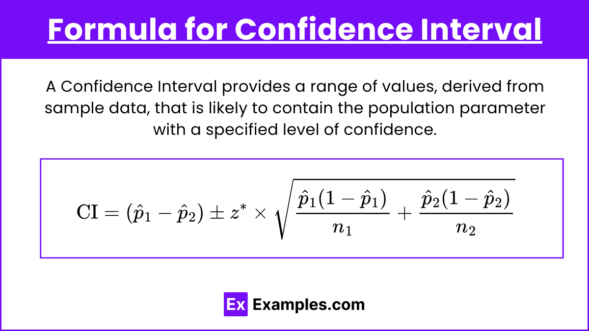
The confidence interval for the difference between two proportions p₁ and p₂ is given by:

\(\text{CI} = (\hat{p}_1 – \hat{p}_2) \pm z^* \times \sqrt{\frac{\hat{p}_1(1-\hat{p}_1)}{n_1} + \frac{\hat{p}_2(1-\hat{p}_2)}{n_2}}\)

Where:

\( \hat{p}_1 \) and \( \hat{p}_2 \) are the sample proportions.
\( n_1 \) and \( n_2 \) are the sample sizes.
\( z^* \)

Steps to Calculate the Confidence Interval

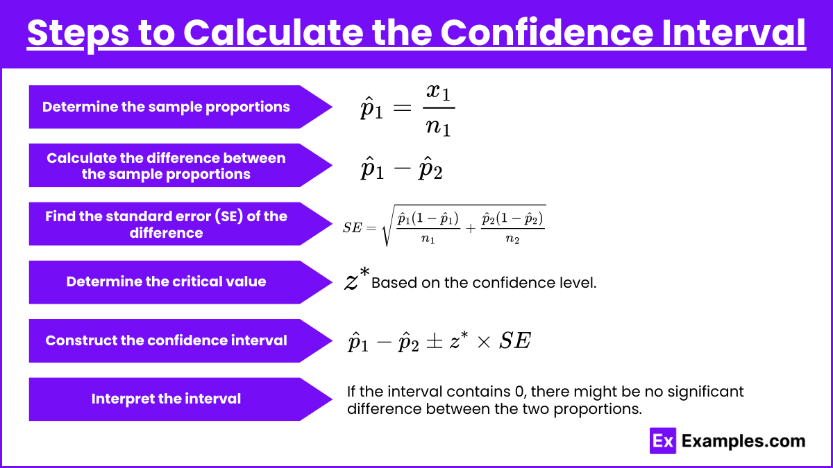
Determine the sample proportions: \( \hat{p}_1 = \frac{x_1}{n_1} \) and \( \hat{p}_2 = \frac{x_2}{n_2} \), where \( x_1 \) and \( x_2 \) are the number of successes in each sample.
Calculate the difference between the sample proportions: \( \hat{p}_1 – \hat{p}_2 \).
Find the standard error (SE) of the difference: \(SE = \sqrt{\frac{\hat{p}_1(1-\hat{p}_1)}{n_1} + \frac{\hat{p}_2(1-\hat{p}_2)}{n_2}}\)
Determine the critical value \( z^* \) based on the confidence level.
Construct the confidence interval: \(\hat{p}_1 – \hat{p}_2) \pm z^* \times SE\)
Interpret the interval: If the interval contains 0, there might be no significant difference between the two proportions.

Hypothesis Tests for the Difference Between Two Proportions

Hypothesis testing is used to determine if the difference between two population proportions is statistically significant.

Null and Alternative Hypotheses

For the difference between two proportions, the hypotheses are generally stated as:

\textbf{Null Hypothesis (H₀):} \( p_1 = p_2 \) or \( p_1 – p_2 = 0 \) (There is no difference between the two population proportions).
\textbf{Alternative Hypothesis (H₁):} \( p_1 \neq p_2\), \( p_1 > p_2 \), or \( p_1 < p_2 \) depending on the context (There is a difference between the two population proportions).

Test Statistic

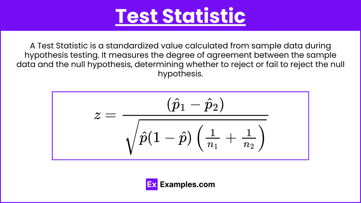
The test statistic for comparing two proportions is given by:

\(z = \frac{(\hat{p}_1 – \hat{p}_2)}{\sqrt{\hat{p}(1-\hat{p})\left(\frac{1}{n_1} + \frac{1}{n_2}\right)}}\)

Where:

\( \hat{p} = \frac{x_1 + x_2}{n_1 + n_2} \) is the pooled proportion.
\( \hat{p}_1 \) and ( \hat{p}_2 \) are the sample proportions.
\( n_1 \) and (\ n_2 \) are the sample sizes.

Steps for Hypothesis Testing

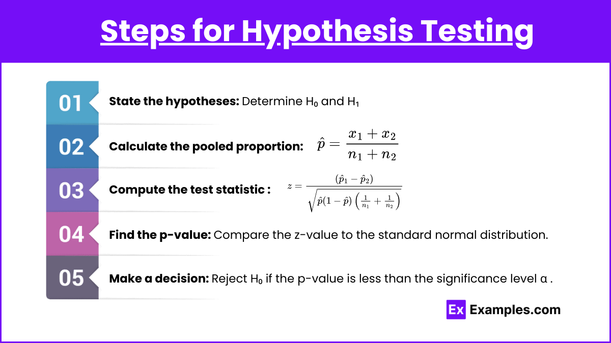
State the hypotheses: Determine \( H_0 \) and \( H_1 \).
Calculate the pooled proportion: \(\hat{p} = \frac{x_1 + x_2}{n_1 + n_2}\)
Compute the test statistic z: \(z = \frac{(\hat{p}_1 – \hat{p}_2)}{\sqrt{\hat{p}(1-\hat{p})\left(\frac{1}{n_1} + \frac{1}{n_2}\right)}}\)
Find the p-value: Compare the z-value to the standard normal distribution.
Make a decision: Reject \(H_0\) if the p-value is less than the significance level α (typically 0.05).

Examples

Example 1:

Scenario: In a survey, 120 out of 200 students at School A support a new policy, while 90 out of 150 students at School B support it. Construct a 95% confidence interval for the difference in proportions.

\( \hat{p}_1 = \frac{120}{200} = 0.60 \)
\( \hat{p}_2 = \frac{90}{150} = 0.60 \)
\( SE = \sqrt{\frac{0.6 \times 0.4}{200} + \frac{0.6 \times 0.4}{150}} \approx 0.05477 \)
\( z^* = 1.96 \) for 95\% confidence

Confidence Interval:\((0.60 – 0.60) \pm 1.96 \times 0.05477 = 0 \pm 0.1074 = (-0.1074, 0.1074)\)

Interpretation: The true difference in proportions could be as much as -10.74% to +10.74%.

Example 2:

Scenario: 70 out of 100 students at School C passed a test, while 85 out of 120 students at School D passed. Test if there is a significant difference at α=0.05.

\( \hat{p}_1 = \frac{70}{100} = 0.70 \)
\( \hat{p}_2 = \frac{85}{120} = 0.7083 \)
\( \hat{p} = \frac{70 + 85}{100 + 120} = 0.7042 \)
\( z = \frac{0.70 – 0.7083}{\sqrt{0.7042 \times 0.2958 \times \left(\frac{1}{100} + \frac{1}{120}\right)}} \approx -0.106 \)

p-value: Greater than 0.05

Decision: Fail to reject \(H_0\), no significant difference.

Example 3:

Scenario: A company finds that 45% of their customers are satisfied in Region X, and 50% are satisfied in Region Y. They sample 400 customers from each region. Compute the 90% confidence interval for the difference in satisfaction rates.

\( \hat{p}_1 = 0.45 \)
\( \hat{p}_2 = 0.50 \)
\( SE = \sqrt{\frac{0.45 \times 0.55}{400} + \frac{0.50 \times 0.50}{400}} \approx 0.0353\)
\( z^* = 1.645 \) for 90\% confidence

Confidence Interval:

\((0.45 – 0.50) \pm 1.645 \times 0.0353 = -0.05 \pm 0.0581 = (-0.1081, 0.0081)\)

Example 4:

Scenario: Two political candidates claim support of 40% and 35% of voters, respectively. If they sample 500 voters each, test for a significant difference at α=0.01\alpha = 0.01α=0.01.

\( \hat{p}_1 = 0.40 \)
\( \hat{p}_2 = 0.35 \)
\( \hat{p} = \frac{0.40 + 0.35}{2} = 0.375 \)
\( z = \frac{0.40 – 0.35}{\sqrt{0.375 \times 0.625 \times \left(\frac{1}{500} + \frac{1}{500}\right)}} \approx 1.69 \)

p-value: Between 0.05 and 0.01

Decision: Fail to reject \(H_0\), not significant at α=0.01\alpha = 0.01α=0.01.

Example 5:

Scenario: In a clinical trial, 15% of patients receiving Drug A showed improvement, while 20% of patients receiving Drug B did. 300 patients were assigned to each group. Construct the 95% confidence interval for the difference in improvement rates.

\( \hat{p}_1 = 0.15 \)
\( \hat{p}_2 = 0.20 \)
\( SE = \sqrt{\frac{0.15 \times 0.85}{300} + \frac{0.20 \times 0.80}{300}} \approx 0.0316 \)
\( z^* = 1.96 \) for 95\% confidence

Confidence Interval:\((0.15 – 0.20) \pm 1.96 \times 0.0316 = -0.05 \pm 0.0619 = (-0.1119, 0.0119)\)

Multiple Choice Questions

MCQ 1:

A 90% confidence interval for the difference between two proportions is calculated as (-0.05, 0.10). What can be concluded?

There is a significant difference between the two proportions.
There is no significant difference between the two proportions.
The two proportions are equal.
The sample size is too small to draw a conclusion.

Answer: 2
Explanation: The interval includes 0, so there is no significant difference.

MCQ 2:

Which of the following is the correct formula for the standard error used in constructing a confidence interval for the difference between two proportions?

\( \sqrt{\frac{\hat{p}_1(1-\hat{p}_1)}{n_1} + \frac{\hat{p}_2(1-\hat{p}_2)}{n_2}} \)
\( \sqrt{\frac{p(1-p)}{n_1} + \frac{p(1-p)}{n_2}} \)
\( \sqrt{p_1 \times p_2} \)
\( \frac{\hat{p}_1 – \hat{p}_2}{SE} \)

Answer: 1
Explanation: The first option is the correct formula for the standard error when comparing two proportions.

MCQ 3:

In hypothesis testing for two proportions, the null hypothesis H0H_0H0 is:

\( p_1 > p_2 \)
\( p_1 < p_2 \)
\( p_1 = p_2 \)
\( p_1 \geq p_2 \)

Answer: 3
Explanation: The null hypothesis typically states that the two population proportions are equal (no difference).