Random Variables and Probability Distributions

Last Updated: September 23, 2024

Notes

In AP Statistics, understanding random variables and probability distributions is crucial. A random variable assigns numerical values to the outcomes of a random phenomenon, while a probability distribution describes how probabilities are distributed over these values. Mastery of these concepts enables students to analyze data, predict outcomes, and make informed decisions. This introduction lays the foundation for exploring discrete and continuous random variables, probability mass functions, and cumulative distribution functions.

Learning Objectives

By studying random variables and probability distributions in AP Statistics, you will understand how to assign numerical values to random phenomena and interpret probability distributions. You will learn to differentiate between discrete and continuous random variables, analyze probability mass functions, and use cumulative distribution functions. This knowledge will help you predict outcomes, make data-driven decisions, and interpret statistical results effectively. Mastering these concepts is essential for your success in statistics and data analysis.

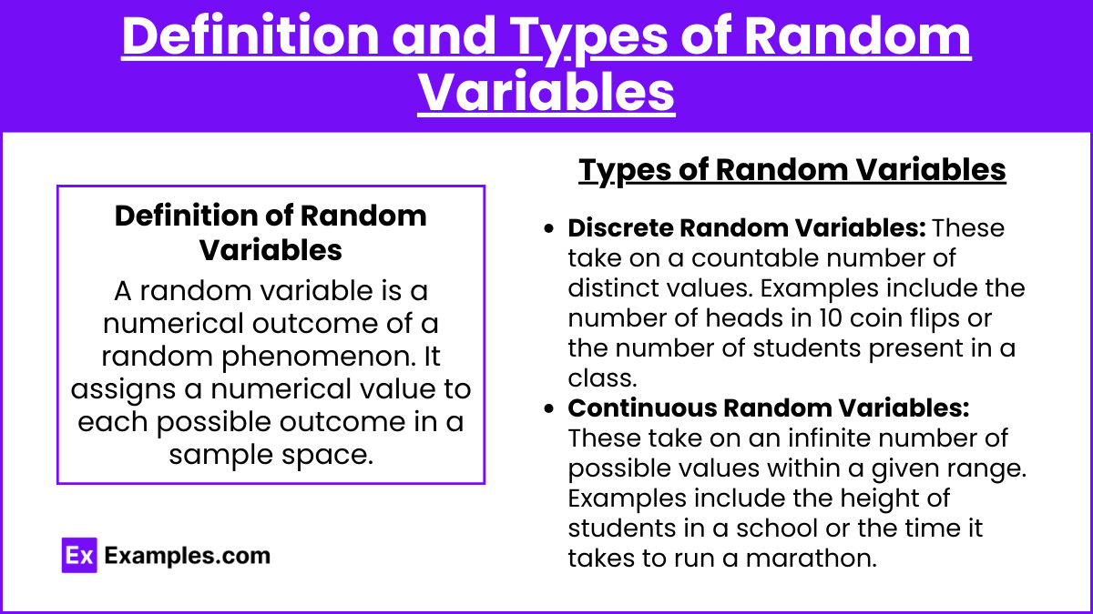
Definition of Random Variables

A random variable is a numerical outcome of a random phenomenon. It assigns a numerical value to each possible outcome in a sample space.

Types of Random Variables

Discrete Random Variables: These take on a countable number of distinct values. Examples include the number of heads in 10 coin flips or the number of students present in a class.
Continuous Random Variables: These take on an infinite number of possible values within a given range. Examples include the height of students in a school or the time it takes to run a marathon.

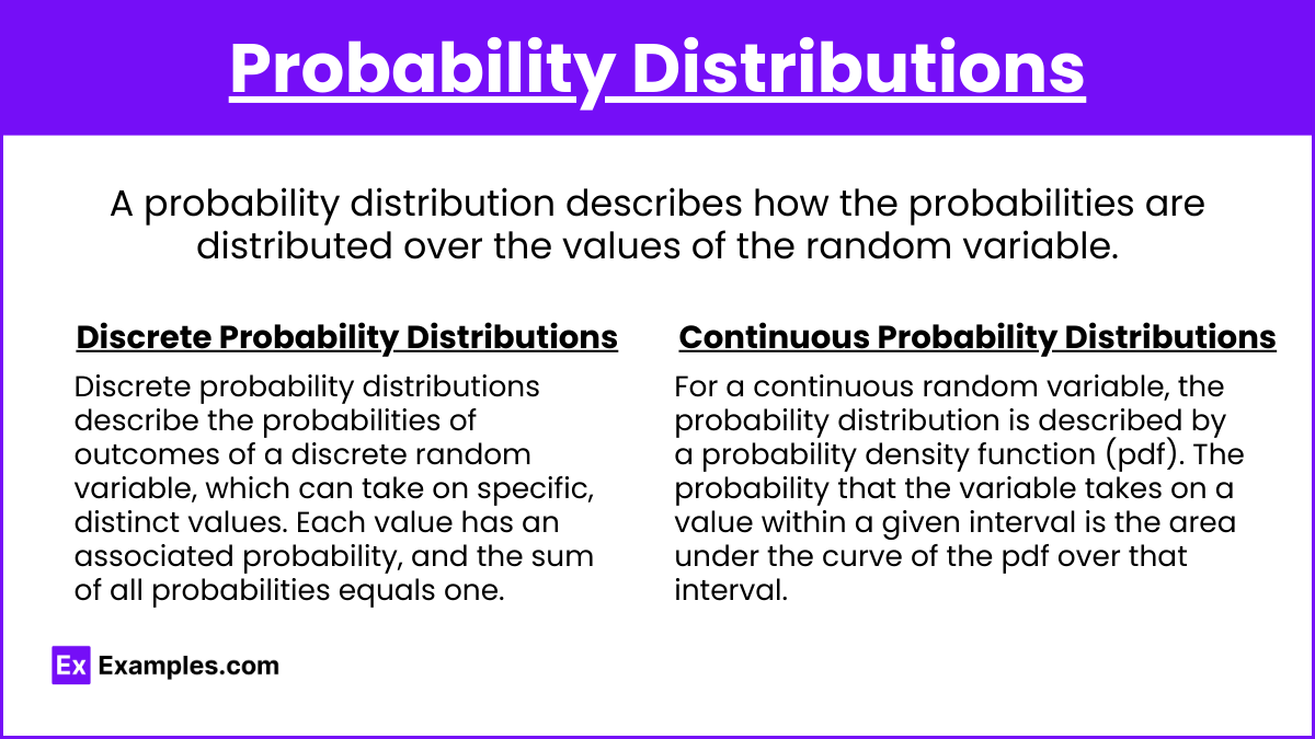
Probability Distributions

A probability distribution describes how the probabilities are distributed over the values of the random variable.

Discrete Probability Distributions

For a discrete random variable, the probability distribution is a list of probabilities associated with each of its possible values.

Example: The probability distribution of rolling a fair six-sided die.

$P(X=1) &= \frac{1}{6}$
$P(X=2) &= \frac{1}{6}$
$P(X=3) &= \frac{1}{6}$
$P(X=4) &= \frac{1}{6}$
$P(X=5) &= \frac{1}{6}$
$P(X=6) &= \frac{1}{6}$

Continuous Probability Distributions

For a continuous random variable, the probability distribution is described by a probability density function (pdf). The probability that the variable takes on a value within a given interval is the area under the curve of the pdf over that interval.

Example: The height of adult males in a certain population might be modeled by a normal distribution with a mean μ\muμ and standard deviation σ\sigmaσ.

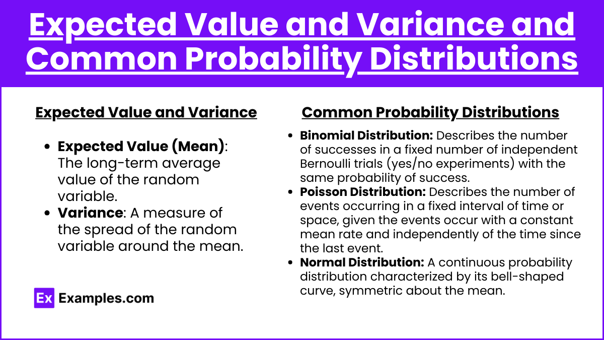
Expected Value and Variance

Expected Value (Mean): The long-term average value of the random variable.
- For a discrete random variable X: $E(X) = \sum [x \cdot P(x)]$
- For a continuous random variable X: $[E(X) = \int_{-\infty}^{\infty} x f(x) \, dx$
Variance: A measure of the spread of the random variable around the mean.
- For a discrete random variable X: $\text{Var}(X) = \sum [(x - E(X))^2 \cdot P(x)]$
- For a continuous random variable X
- $[\text{Var}(X) = \int_{-\infty}^{\infty} (x - E(X))^2 f(x) \, dx$

Common Probability Distributions

Binomial Distribution: Describes the number of successes in a fixed number of independent Bernoulli trials (yes/no experiments) with the same probability of success.
Poisson Distribution: Describes the number of events occurring in a fixed interval of time or space, given the events occur with a constant mean rate and independently of the time since the last event.
Normal Distribution: A continuous probability distribution characterized by its bell-shaped curve, symmetric about the mean.

Examples

Example 1: Discrete Random Variable (Dice Roll)
- A six-sided die is rolled. Let XXX be the number on the die.
- Probability Distribution:
- $P(X = k) = \frac{1}{6} \quad \text{for} \quad k = 1, 2, 3, 4, 5, 6$
- Expected Value: $E(X) = \sum_{k=1}^{6} k \cdot \frac{1}{6} = 3.5$
- Variance: Var(X)= $\text{Var}(X) = \sum_{k=1}^{6} (k - 3.5)^2 \cdot \frac{1}{6} = 2.92$
Example 2: Continuous Random Variable (Uniform Distribution)
- The time TTT to complete a task is uniformly distributed between 30 and 60 minutes.
- Probability Density Function: f(t)=130f(t) = [ f(t) = $\frac{1}{30} \quad \text{for} \quad 30 \leq t \leq 60$
- Expected Value: $E(T) = \frac{30 + 60}{2} = 45$
- Variance: Var(T)= $\text{Var}(T) = \frac{(60 - 30)^2}{12} = 75$
Example 3: Binomial Distribution
- Flipping a coin 10 times, with XXX representing the number of heads.
- Probability Distribution: $P(X = k) = \binom{10}{k} (0.5)^{10}$
- Expected Value: $E(X) = 10 \cdot 0.5 = 5$
- Variance: $\text{Var}(X) = 10 \cdot 0.5 \cdot 0.5 = 2.5$
Example 4: Poisson Distribution
- The number of emails received per hour follows a Poisson distribution with a mean of 3.
- Probability Distribution: $P(X = k) = \frac{3^k e^{-3}}{k!}$ .
- Expected Value: $E(X) = 3$
- Variance: $\text{Var}(X) = 3$
Example 5: Normal Distribution
- Heights of students in a school follow a normal distribution with mean 65 inches and standard deviation 3 inches.
- Probability Density Function:[ f(x) = $\frac{1}{3\sqrt{2\pi}} e^{-\frac{(x - 65)^2}{18}}$
- Expected Value: $E(X) = 65$ .
- Variance: $\text{Var}(X) = 9$

Multiple Choice Questions (MCQs)

Question 1: Which of the following is true for a normal distribution?

A) The mean, median, and mode are all equal.
B) The mean is always greater than the median.
C) The distribution is skewed to the right.
D) The variance is always zero.

Answer: A) The mean, median, and mode are all equal.

Explanation: In a normal distribution, the mean, median, and mode are all located at the center of the distribution, making them equal.

Question 2: If a random variable XXX follows a binomial distribution with parameters n=10n = 10n=10 and p=0.5p = 0.5p=0.5, what is the expected value of XXX?

A) 2.5
B) 5
C) 7.5
D) 10

Answer: B) 5

Explanation: The expected value of a binomial random variable XXX is given by E(X)=npE(X) = npE(X)=np. Here, E(X)=10×0.5=5E(X) = 10 \times 0.5 = 5E(X)=10×0.5=5.

Question 3: For a continuous random variable with a uniform distribution over the interval [a, b], what is the probability density function (pdf)?

A) $\frac{1}{b-a} for a \leq x \leq b$
B) $\frac{x-a}{b-a}$
C) $\frac{b-x}{b-a}$
D) $\frac{1}{b+a}$

Answer: A) $f(x)=1b−f(x) = \frac{1}{b-a} for a \leq x \leq b$

Explanation: For a uniform distribution over the interval [a, b], the probability density function (pdf) is constant and equal to $\frac{1}{b-a}.$ .