
Residuals and Residual Plots

![\[\text{Residual} = \text{Observed value} - \text{Predicted value}\]](https://www.examples.com/wp-content/ql-cache/quicklatex.com-33264c9a6d076388e81776518bd4b0bb_l3.svg "Rendered by QuickLaTeX.com")
![\[\text{Observed values: } y = [4, 5, 6, 7, 8] \]](https://www.examples.com/wp-content/ql-cache/quicklatex.com-2330082de64dd335407fe7107185eb11_l3.svg "Rendered by QuickLaTeX.com")
![\[\text{Predicted values from the model: } \hat{y} = [3.8, 5.1, 6.3, 6.9, 8.2]\]](https://www.examples.com/wp-content/ql-cache/quicklatex.com-d06233bf50e0c9d16225c11f95cfc492_l3.svg "Rendered by QuickLaTeX.com")
![\[\text{Residuals} = [4 - 3.8, 5 - 5.1, 6 - 6.3, 7 - 6.9, 8 - 8.2] = [0.2, -0.1, -0.3, 0.1, -0.2]\]](https://www.examples.com/wp-content/ql-cache/quicklatex.com-9fd9c817818e1a3e63b7b86698ed39eb_l3.svg "Rendered by QuickLaTeX.com")
![\[\hat{y} = 2x + 1\]](https://www.examples.com/wp-content/ql-cache/quicklatex.com-365e6464f75b08be03c7b1d6e4a8977b_l3.svg "Rendered by QuickLaTeX.com")
![\[\hat{y} = [3, 5, 7, 9, 11]\]](https://www.examples.com/wp-content/ql-cache/quicklatex.com-e0de5dd8c7b5290ee9a6866302322d87_l3.svg "Rendered by QuickLaTeX.com")
![\[\text{Residuals} = [4 - 3, 5 - 5, 7 - 7, 8 - 9, 11 - 11] = [1, 0, 0, -1, 0]\]](https://www.examples.com/wp-content/ql-cache/quicklatex.com-307718c28ca2562033def5fb3ce67c9b_l3.svg "Rendered by QuickLaTeX.com")
![\[(x, y) = (2, 4), (4, 5), (6, 6), (8, 8), (10, 9)\]](https://www.examples.com/wp-content/ql-cache/quicklatex.com-f88817864d6392bcf3b3b2f0fb922837_l3.svg "Rendered by QuickLaTeX.com")
![\[\hat{y} = [4, 5, 6, 7, 8]\]](https://www.examples.com/wp-content/ql-cache/quicklatex.com-6f9d200d543135dd08f8cfd930ee2316_l3.svg "Rendered by QuickLaTeX.com")
![\[\text{Residuals} = [4 - 4, 5 - 5, 6 - 6, 8 - 7, 9 - 8] = [0, 0, 0, 1, 1]\]](https://www.examples.com/wp-content/ql-cache/quicklatex.com-5f14a59497f6348932da65d645e964e0_l3.svg "Rendered by QuickLaTeX.com")
![\[\hat{y} = 0.6x + 2\]](https://www.examples.com/wp-content/ql-cache/quicklatex.com-cc4a01a448d03e78b2b997b67588014b_l3.svg "Rendered by QuickLaTeX.com")
![\[(x, y) = (3, 3), (5, 5), (7, 8), (9, 10), (11, 11)\]](https://www.examples.com/wp-content/ql-cache/quicklatex.com-64bf04696090b690c0933932b2fa850f_l3.svg "Rendered by QuickLaTeX.com")
![\[ \hat{y} = [3.8, 5.8, 7.8, 9.8, 11.8]\]](https://www.examples.com/wp-content/ql-cache/quicklatex.com-c93186e8c64b00153df321f3990bd940_l3.svg "Rendered by QuickLaTeX.com")
![\[\text{Residuals} = [3 - 3.8, 5 - 5.8, 8 - 7.8, 10 - 9.8, 11 - 11.8] = [-0.8, -0.8, 0.2, 0.2, -0.8]\]](https://www.examples.com/wp-content/ql-cache/quicklatex.com-2294878c5ca6b7d3d0c51fdfd1873b1b_l3.svg "Rendered by QuickLaTeX.com")
![\[\text{Observed: } y = [1, 4, 9, 16, 25] \\]](https://www.examples.com/wp-content/ql-cache/quicklatex.com-28bb7b1243309a90af697b40c0340505_l3.svg "Rendered by QuickLaTeX.com")
![\[\text{Predicted: } \hat{y} = [1, 3, 8, 15, 24]\]](https://www.examples.com/wp-content/ql-cache/quicklatex.com-aaf7b53e968319731e8044ef4f03e5f2_l3.svg "Rendered by QuickLaTeX.com")
![\[\text{Residuals} = [0, 1, 1, 1, 1]\]](https://www.examples.com/wp-content/ql-cache/quicklatex.com-0e984a4398dcec36f0d6370f23ae439b_l3.svg "Rendered by QuickLaTeX.com")
In AP Statistics, understanding residuals and residual plots is crucial for evaluating regression models. Residuals are the differences between observed and predicted values, indicating the model's accuracy. Residual plots graph these differences, helping to assess linearity, homoscedasticity, and independence. Analyzing these plots ensures the model fits the data well and identifies any patterns or anomalies. Mastering these concepts is essential for interpreting and improving statistical models, a key skill for excelling in AP Statistics.
Learning Objectives
By studying residuals and residual plots, I will learn how to evaluate the accuracy and fit of regression models in AP Statistics. I will understand how to calculate residuals and create residual plots to identify patterns and anomalies. This knowledge will help me assess linearity, homoscedasticity, and independence in data. Mastering these skills will enable me to interpret and improve statistical models effectively, enhancing my overall proficiency in AP Statistics.
Definition of Residuals
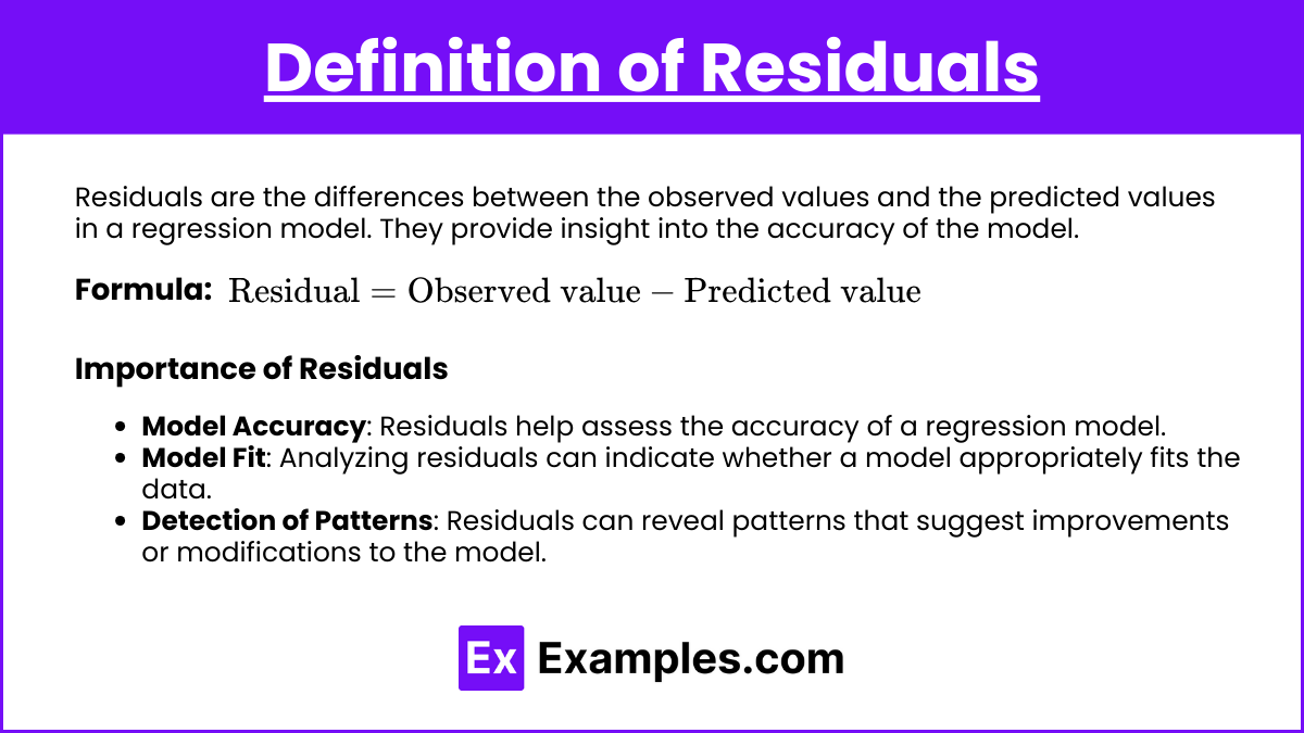
Residuals are the differences between the observed values and the predicted values in a regression model. They provide insight into the accuracy of the model.
Formula:
\text{Residual} = \text{Observed value} - \text{Predicted value}
Importance of Residuals
Model Accuracy: Residuals help assess the accuracy of a regression model.
Model Fit: Analyzing residuals can indicate whether a model appropriately fits the data.
Detection of Patterns: Residuals can reveal patterns that suggest improvements or modifications to the model.
Definition of Residual Plots
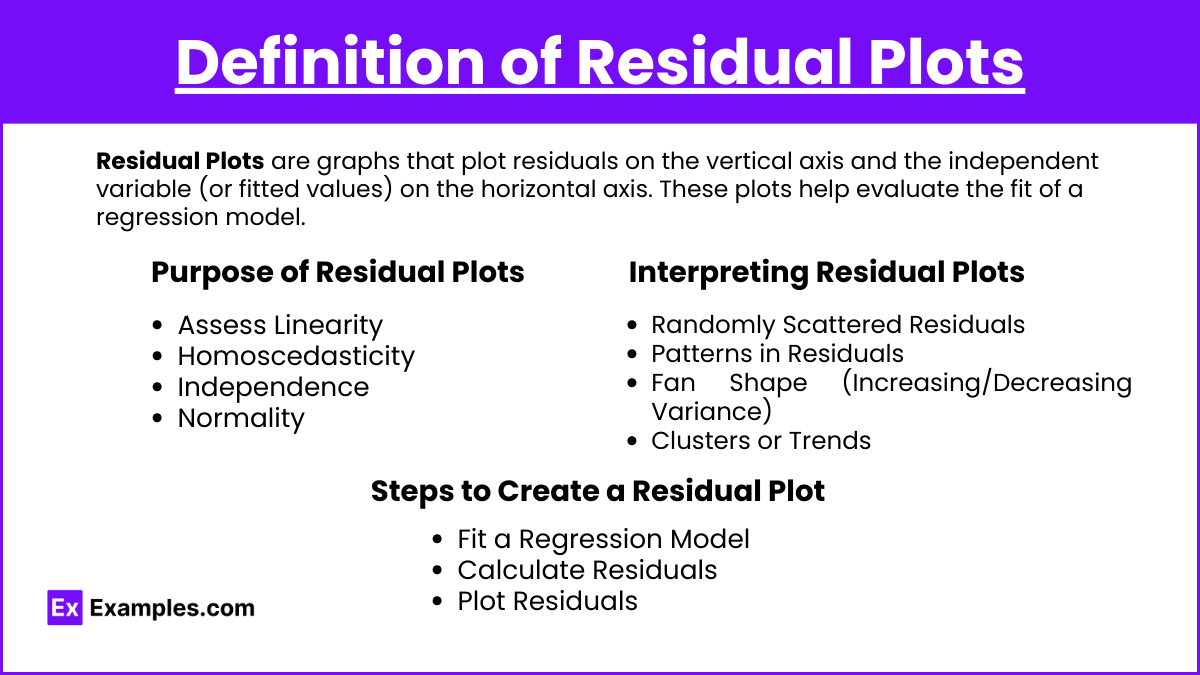
Residual Plots are graphs that plot residuals on the vertical axis and the independent variable (or fitted values) on the horizontal axis. These plots help evaluate the fit of a regression model.
Purpose of Residual Plots
Assess Linearity: Check if the relationship between variables is linear.
Homoscedasticity: Evaluate if the residuals have constant variance.
Independence: Determine if residuals are independent of each other.
Normality: Check if residuals are approximately normally distributed.
Interpreting Residual Plots
Randomly Scattered Residuals: Suggests a good fit for a linear model.
Patterns in Residuals: Indicates potential problems with the model, such as non-linearity or heteroscedasticity.
Fan Shape (Increasing/Decreasing Variance): Indicates heteroscedasticity.
Clusters or Trends: Suggests that the model may not have captured some underlying patterns in the data.
Steps to Create a Residual Plot
Fit a Regression Model: Use statistical software or a calculator to fit a regression line to the data.
Calculate Residuals: Compute the residuals for each data point.
Plot Residuals: Create a scatter plot with residuals on the y-axis and the independent variable (or fitted values) on the x-axis.
Examples
Example 1
Consider the data set:
\text{Observed values: } y = [4, 5, 6, 7, 8]
\text{Predicted values from the model: } \hat{y} = [3.8, 5.1, 6.3, 6.9, 8.2]
Residuals:
\text{Residuals} = [4 - 3.8, 5 - 5.1, 6 - 6.3, 7 - 6.9, 8 - 8.2] = [0.2, -0.1, -0.3, 0.1, -0.2]
Example 2
Given the regression model \hat{y} = 2x + 1 and data points:
(x, y) = (1, 4), (2, 5), (3, 7), (4, 8), (5, 11)
Predicted values: \hat{y} = [3, 5, 7, 9, 11]
Residuals:
\text{Residuals} = [4 - 3, 5 - 5, 7 - 7, 8 - 9, 11 - 11] = [1, 0, 0, -1, 0]
Example 3
For a regression model \hat{y} = 3 + 0.5x and data points:
(x, y) = (2, 4), (4, 5), (6, 6), (8, 8), (10, 9)
Predicted values: \hat{y} = [4, 5, 6, 7, 8]
Residuals:
\text{Residuals} = [4 - 4, 5 - 5, 6 - 6, 8 - 7, 9 - 8] = [0, 0, 0, 1, 1]
Example 4
For a regression line \hat{y} = 0.6x + 2 and data:
(x, y) = (3, 3), (5, 5), (7, 8), (9, 10), (11, 11)
Predicted values: \hat{y} = [3.8, 5.8, 7.8, 9.8, 11.8]
Residuals:
\text{Residuals} = [3 - 3.8, 5 - 5.8, 8 - 7.8, 10 - 9.8, 11 - 11.8] = [-0.8, -0.8, 0.2, 0.2, -0.8]
Example 5
Given a dataset with a quadratic relationship, the residuals might look different:
\text{Observed: } y = [1, 4, 9, 16, 25] \
\text{Predicted: } \hat{y} = [1, 3, 8, 15, 24]
Residuals: \text{Residuals} = [0, 1, 1, 1, 1]
Multiple Choice Questions
MCQ 1
Which of the following indicates a good fit in a residual plot?
A distinct pattern.
Randomly scattered residuals.
A U-shaped pattern.
Residuals increasing with the independent variable.
Answer: 2. Randomly scattered residuals.
Explanation: Randomly scattered residuals suggest that the model's errors are randomly distributed, indicating a good fit.
MCQ 2
If residuals show a fan shape, this indicates:
Linearity.
Heteroscedasticity.
Independence.
Homoscedasticity.
Answer: 2. Heteroscedasticity.
Explanation: A fan shape in the residual plot indicates that the variance of the residuals changes with the independent variable, a condition known as heteroscedasticity.
MCQ 3
In a residual plot, what does it mean if there is a clear pattern?
The model perfectly fits the data.
The model has not captured all the underlying trends.
Residuals are normally distributed.
The residuals are homoscedastic.
Answer: 2. The model has not captured all the underlying trends.
Explanation: A clear pattern in a residual plot indicates that the model may be missing some aspect of the relationship between the independent and dependent variables.