The Central Limit Theorem

In AP Statistics, the Central Limit Theorem (CLT) is a fundamental concept that states the sampling distribution of the sample mean approaches a normal distribution as the sample size increases, regardless of the population’s distribution. This theorem allows students to make inferences about population parameters using sample statistics. By understanding the CLT, you will be able to apply normal probability methods to various statistical problems, making it a crucial tool for accurate data analysis and interpretation.

Learning Objectives

By studying the Central Limit Theorem in AP Statistics, you will understand how the sampling distribution of the sample mean approaches a normal distribution as the sample size increases. You will learn to apply this theorem to make inferences about population parameters using sample data. This knowledge will help you use normal probability methods in various statistical problems, enhancing your ability to analyze and interpret data accurately and effectively. Mastering the CLT is essential for success in statistics.

Definition and Key Concepts

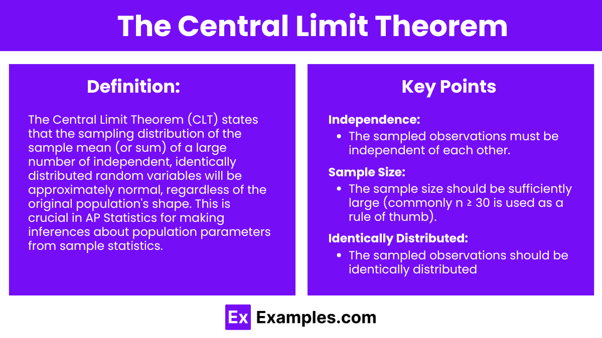
The Central Limit Theorem (CLT) is a fundamental theorem in statistics that states that the sampling distribution of the sample mean (or sum) of a sufficiently large number of independent, identically distributed random variables will be approximately normally distributed, regardless of the shape of the original population distribution. This theorem is crucial in AP Statistics for making inferences about population parameters based on sample statistics.

Key Points

1. Independence: The sampled observations must be independent of each other.
2. Sample Size: The sample size should be sufficiently large (commonly n ≥ 30 is used as a rule of thumb).
3. Identically Distributed: The sampled observations should be identically distributed (i.e., drawn from the same population with the same distribution).

Central Limit Theorem for Sample Means

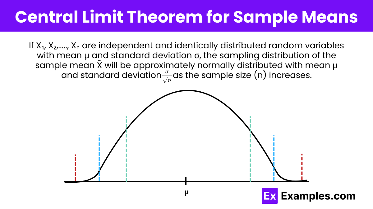
• If \(X_1, X_2, \ldots, X_n\) are independent and identically distributed random variables with mean \(\mu\) and standard deviation \(\sigma\), the sampling distribution of the sample mean \(\bar{X}\) will be approximately normally distributed with mean \(\mu\) and standard deviation \(\frac{\sigma}{\sqrt{n}}\) as the sample size (n) increases.

Central Limit Theorem for Sums

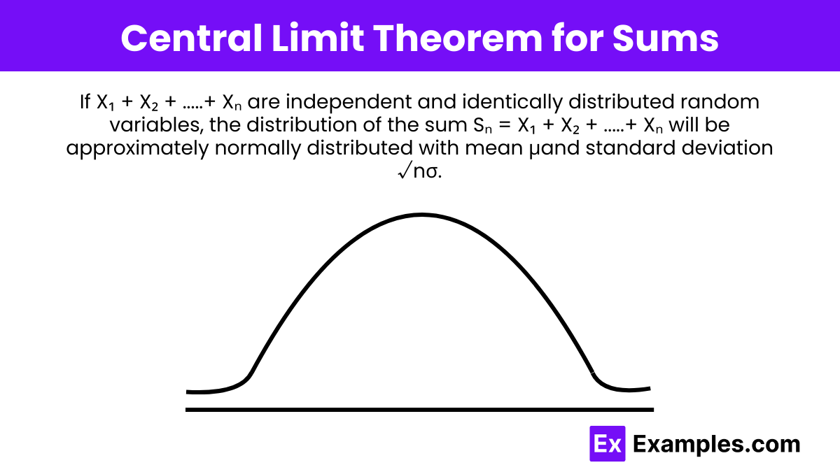
• If \(X_1 + X_2 + \cdots + X_n\) are independent and identically distributed random variables, the distribution of the sum \(S_n = X_1 + X_2 + \cdots + X_n\) will be approximately normally distributed with mean \(\mu\) and standard deviation \(\sqrt{n}\sigma\).

Importance in Statistics

The CLT allows us to:

• Use the normal distribution to approximate the sampling distribution of the sample mean or sum, even when the population distribution is not normal.
• Construct confidence intervals and perform hypothesis tests for population parameters.

Examples

Example 1: Rolling Dice

Suppose you roll a six-sided die 50 times and calculate the mean of the outcomes. According to the CLT, the sampling distribution of the mean will be approximately normal, even though the population distribution (outcomes of a die roll) is uniform.

Example 2: Survey Responses

A survey asks respondents to rate their satisfaction on a scale from 1 to 10. If we take random samples of 40 respondents each, the mean satisfaction score of each sample will be approximately normally distributed, regardless of the original satisfaction score distribution.

Example 3: Quality Control

In a factory, the length of bolts produced is measured. The length follows an unknown distribution with a mean of 5 cm and a standard deviation of 0.2 cm. If we take samples of 100 bolts each, the sampling distribution of the mean length will be approximately normal.

Example 4: Heights of Students

The heights of students in a school are not normally distributed. However, if we take random samples of 35 students each and calculate the mean height, the distribution of the sample means will be approximately normal due to the CLT.

Example 5: Stock Returns

Daily returns of a particular stock are highly skewed. If we take samples of 50 days each and compute the average return, the distribution of these average returns will be approximately normal according to the CLT.

Multiple Choice Questions (MCQs)

MCQ 1

Which of the following best describes the Central Limit Theorem?

A. The population distribution becomes normal as the sample size increases.
B. The sample mean distribution becomes normal regardless of the sample size.
C. The sample mean distribution approaches a normal distribution as the sample size increases.
D. The variance of the sample mean increases with sample size.

Answer: C
Explanation: The CLT states that the distribution of the sample mean approaches a normal distribution as the sample size increases, regardless of the shape of the population distribution.

MCQ 2

If the population mean is 50 and the population standard deviation is 10, what is the standard deviation of the sample mean for samples of size 25?

A. 10
B. 2
C. 5
D. 20

Answer: B
Explanation:

The standard deviation of the sample mean \(\sigma_{\bar{X}}\) is given by \(\frac{\sigma}{\sqrt{n}}\). Here, \(\sigma = 10) and (n = 25\), so
\(
\sigma_{\bar{X}} = \frac{10}{\sqrt{25}} = 2
\)

MCQ 3

Why is the Central Limit Theorem important in statistics?

A. It allows us to assume that the population is normally distributed.
B. It enables us to use normal probability methods to make inferences about the population mean.
C. It shows that the sample mean is equal to the population mean.
D. It indicates that larger samples have more variability.

Answer: B
Explanation: The CLT is important because it allows us to use normal probability methods to make inferences about the population mean, even when the population distribution is not normal.