
The Chi-Square Test for Goodness of Fit

In AP Statistics, the Chi-Square Test for Goodness of Fit is a crucial tool used to determine whether a sample of categorical data matches an expected distribution. This test is particularly useful when you want to assess how well observed frequencies across different categories align with theoretical expectations. By comparing the observed data with the expected frequencies, this test helps determine if any significant deviations exist, indicating that the data may not follow the expected distribution. Understanding and applying the Chi-Square Test for Goodness of Fit is essential for analyzing categorical data and making informed statistical conclusions in various contexts.
Learning Objectives
You will be introduced to the concept and application of the Chi-Square Test for Goodness of Fit. The objective is for you to gain the ability to determine if observed categorical data matches an expected distribution. You will learn how to formulate hypotheses, calculate expected frequencies, compute the Chi-Square statistic, and interpret results. By mastering these skills, you will be able to apply the test in various real-world scenarios, ensuring a solid understanding of categorical data analysis.
What is the Chi-Square Test for Goodness of Fit?
The Chi-Square Test for Goodness of Fit is a statistical method used to determine whether a set of observed categorical data fits a particular distribution. This test compares the observed frequencies of categories to the expected frequencies, based on a specified theoretical distribution. The goal is to assess whether the observed deviations from the expected values are due to random chance or if they are statistically significant.
When to Use the Chi-Square Test for Goodness of Fit
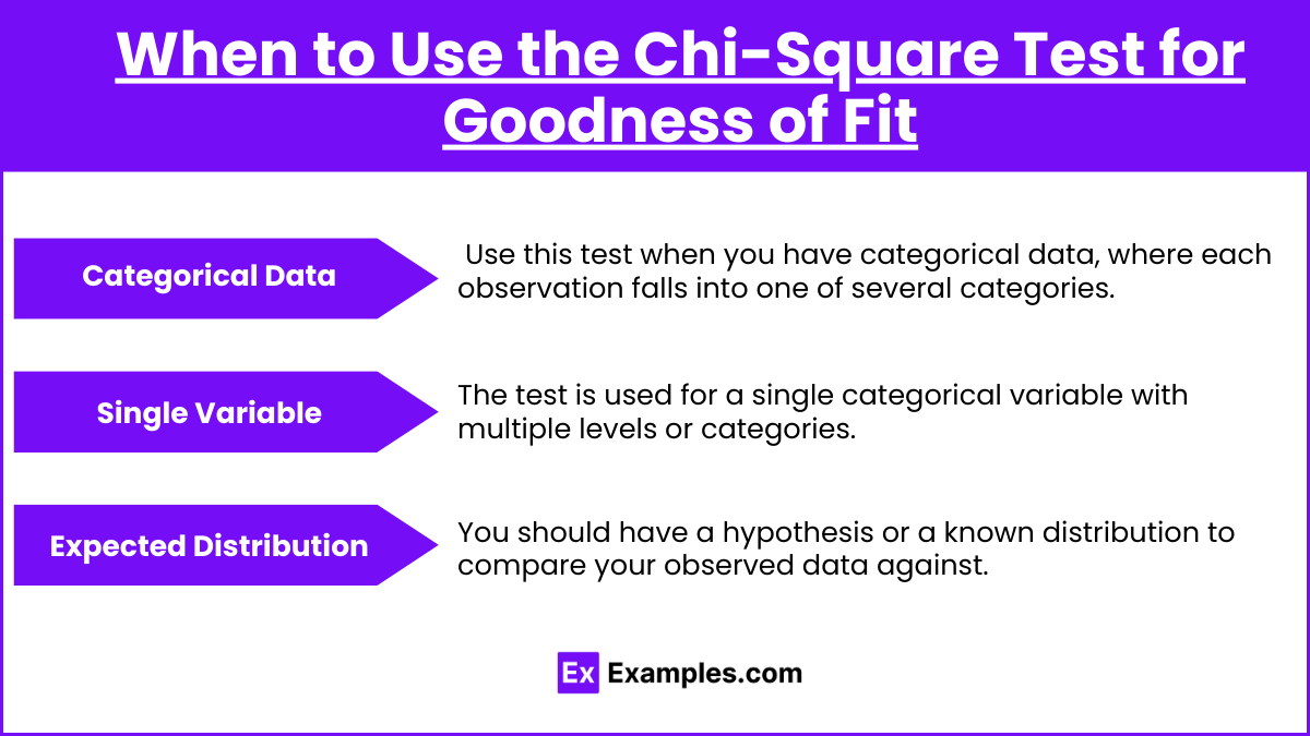
- Categorical Data: Use this test when you have categorical data, where each observation falls into one of several categories.
- Single Variable: The test is used for a single categorical variable with multiple levels or categories.
- Expected Distribution: You should have a hypothesis or a known distribution to compare your observed data against.
Hypotheses in the Chi-Square Test
- Null Hypothesis (H₀): The observed data follows the expected distribution.
- Alternative Hypothesis (H₁): The observed data does not follow the expected distribution.
Formula for Chi-Square Test Statistic
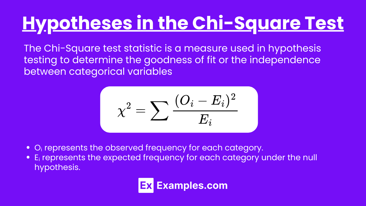
The Chi-Square test statistic (χ²) is calculated using the formula:

- Oᵢ: Observed frequency for category i.
- Eᵢ: Expected frequency for category i.
Steps for Conducting the Chi-Square Test for Goodness of Fit
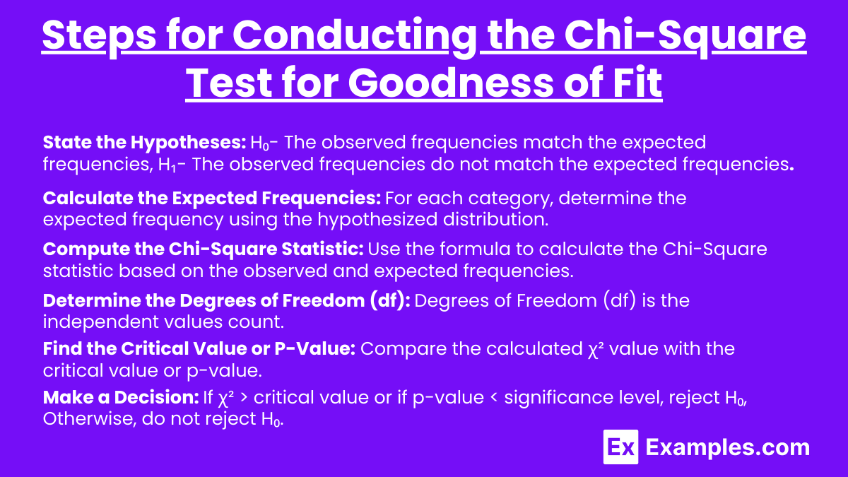
- State the Hypotheses:
- H₀: The observed frequencies match the expected frequencies.
- H₁: The observed frequencies do not match the expected frequencies.
- Calculate the Expected Frequencies:
For each category, determine the expected frequency using the hypothesized distribution.
- Compute the Chi-Square Statistic:
Use the formula to calculate the Chi-Square statistic based on the observed and expected frequencies. - Determine the Degrees of Freedom (df):
Degrees of freedom is calculated as:
where k is the number of categories. - Find the Critical Value or P-Value:
Compare the calculated χ² value with the critical value from the Chi-Square distribution table (based on your significance level, usually 0.05, and degrees of freedom) or find the p-value. - Make a Decision:
- If χ² > critical value or if p-value < significance level, reject H₀.
- Otherwise, do not reject H₀.
Example Scenarios for Chi-Square Test for Goodness of Fit
- Distribution of Colors in a Bag of Candy:
Suppose a candy company claims that the colors in a bag of candies are equally distributed. You can use the Chi-Square test to see if the observed color distribution in a sample bag fits the expected equal distribution. - Genetic Inheritance:
In genetics, the expected ratio of offspring with certain traits might follow Mendelian inheritance patterns (e.g., 3:1 for dominant vs. recessive traits). The Chi-Square test can be used to see if the observed frequencies match the expected ratio. - Customer Preferences:
A company might expect a certain percentage of customers to prefer different flavors of a product. The Chi-Square test can verify if actual preferences match these expectations.
Examples
Example 1:
A die is rolled 60 times, and the outcomes are recorded. The results are as follows: 1 (10 times), 2 (8 times), 3 (12 times), 4 (9 times), 5 (11 times), and 6 (10 times). Test if the die is fair at a 5% significance level.
Solution:
- H₀: The die is fair, meaning each face should appear with equal probability (1/6).
- H₁: The die is not fair.
- Expected Frequency (Eᵢ):

- Observed Frequencies (Oᵢ): 10, 8, 12, 9, 11, 10
- Calculate χ²:
 ]
] - Degrees of Freedom: df = 6 – 1 = 5
- Critical Value (5%, df = 5): 11.07
- Conclusion: Since 1.4 < 11.07, we fail to reject H₀. The die appears to be fair.
Example 2:
A genetics experiment expects a 3:1 ratio of dominant to recessive traits. In a sample of 200 plants, 152 exhibit the dominant trait, and 48 exhibit the recessive trait. Is the observed distribution significantly different from the expected 3:1 ratio?
Solution:
- H₀: The observed distribution fits a 3:1 ratio.
- H₁: The observed distribution does not fit a 3:1 ratio.
- Expected Frequencies: Dominant:
 , Recessive:
- Observed Frequencies: Dominant: 152, Recessive: 48
- Calculate χ²:

- Degrees of Freedom: df = 2 – 1 = 1
- Critical Value (5%, df = 1): 3.84
- Conclusion: Since 0.1333 < 3.84, we fail to reject H₀. The observed data fits the expected 3:1 ratio.
Example 3:
A company claims that 30% of people prefer product A, 50% prefer product B, and 20% prefer product C. A survey of 100 customers shows 25 prefer A, 55 prefer B, and 20 prefer C. Test the company’s claim at a 0.05 significance level.
Solution:
- H₀: The preference distribution is 30%, 50%, and 20%.
- H₁: The preference distribution is different.
- Expected Frequencies: A: 30, B: 50, C: 20
- Observed Frequencies: A: 25, B: 55, C: 20
- Calculate χ²:

- Degrees of Freedom: df = 3 – 1 = 2
- Critical Value (5%, df = 2): 5.99
- Conclusion: Since 1.333 < 5.99, we fail to reject H₀. The survey data supports the company’s claim.
Example 4:
A teacher expects the grades in her class to be normally distributed, with 20% A’s, 30% B’s, 30% C’s, 10% D’s, and 10% F’s. She checks a sample of 100 grades and finds: 15 A’s, 25 B’s, 35 C’s, 15 D’s, and 10 F’s. Is the grade distribution as expected?
Solution:
- H₀: The grades are distributed as 20% A’s, 30% B’s, 30% C’s, 10% D’s, and 10% F’s.
- H₁: The grade distribution is different.
- Expected Frequencies: A: 20, B: 30, C: 30, D: 10, F: 10
- Observed Frequencies: A: 15, B: 25, C: 35, D: 15, F: 10
- Calculate χ²:

- Degrees of Freedom: df = 5 – 1 = 4
- Critical Value (5%, df = 4): 9.49
- Conclusion: Since 5.416 < 9.49, we fail to reject H₀. The grade distribution is as expected.
Example 5:
An astrologer claims that 25% of people are born under each of the four zodiac elements (Fire, Earth, Air, Water). A random sample of 1200 people shows the following distribution: Fire (310), Earth (280), Air (330), Water (280). Test the astrologer’s claim.
Solution:
- H₀: Each zodiac element has a 25% distribution.
- H₁: The distribution differs from 25% each.
- Expected Frequencies:
 for each element.
 - Observed Frequencies: Fire: 310, Earth: 280, Air: 330, Water: 280
- Calculate χ²:

- Degrees of Freedom: df = 4 – 1 = 3
- Critical Value (5%, df = 3): 7.815
- Conclusion: Since 6 < 7.815, we fail to reject H₀. The sample supports the astrologer’s claim.
Multiple Choice Questions (MCQs)
- What is the Chi-Square Test for Goodness of Fit used for?
- a) To compare means between two groups.
- b) To determine if observed frequencies differ from expected frequencies.
- c) To test the correlation between two variables.
- d) To assess the variance of a population.
Explanation: The Chi-Square Test for Goodness of Fit is specifically used to compare observed data with an expected distribution. - Which of the following is true about the degrees of freedom in a Chi-Square Test for Goodness of Fit?
- a) It is the total number of observations.
- b) It is the number of categories minus one.
- c) It is the square of the test statistic.
- d) It is always equal to the number of categories.
Explanation: Degrees of freedom in a Chi-Square Test for Goodness of Fit is calculated as the number of categories minus one. - If a Chi-Square Test for Goodness of Fit yields a p-value of 0.03, what can you conclude at the 0.05 significance level?
- a) There is strong evidence to reject the null hypothesis.
- b) There is not enough evidence to reject the null hypothesis.
- c) The null hypothesis is true.
- d) The alternative hypothesis is false.
Explanation: A p-value of 0.03 is less than the significance level of 0.05, indicating that the observed data significantly differs from the expected distribution.