
The Geometric Distribution


 . What is the probability that the first 4 appears on the 3rd roll?


In AP Statistics, the geometric distribution is vital for modeling the number of trials needed to achieve the first success in a sequence of independent Bernoulli trials. Each trial has a constant probability of success. This distribution helps students understand and calculate the likelihood of various outcomes, such as the first success occurring on a specific trial. Mastery of the geometric distribution enhances problem-solving skills in contexts like quality control, games, and surveys.
Learning Objectives
By studying the geometric distribution in AP Statistics, you will learn to model the number of trials needed for the first success in a series of independent Bernoulli trials. You will understand how to calculate probabilities for specific trials and interpret these probabilities in real-world scenarios. This knowledge will help you solve problems in areas like quality control, gaming strategies, and customer service. Mastering the geometric distribution will enhance your statistical analysis skills and your ability to make data-driven decisions.
Definition and Key Concepts
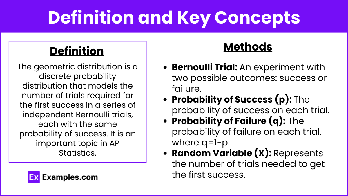
The geometric distribution is a discrete probability distribution that models the number of trials required for the first success in a series of independent Bernoulli trials, each with the same probability of success. It is an important topic in AP Statistics.
Key Properties
Bernoulli Trial: An experiment with two possible outcomes: success or failure.
Probability of Success (p): The probability of success on each trial.
Probability of Failure (q): The probability of failure on each trial, where q=1−p.
Random Variable (X): Represents the number of trials needed to get the first success.
Geometric Probability Formula
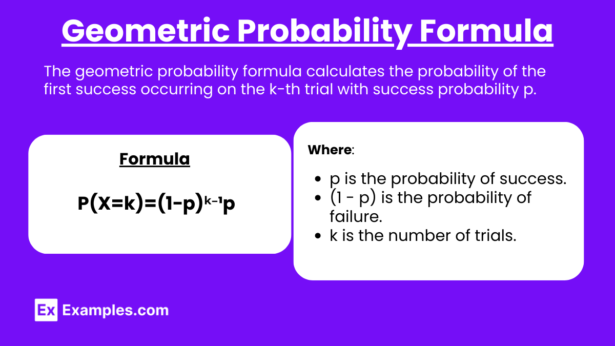
The probability that the first success occurs on the kth trial is given by:
P(X=k)=(1−p)ᵏ⁻¹p
Where:
p is the probability of success.
(1 - p) is the probability of failure.
k is the number of trials.
Mean and Variance of Geometric Distribution
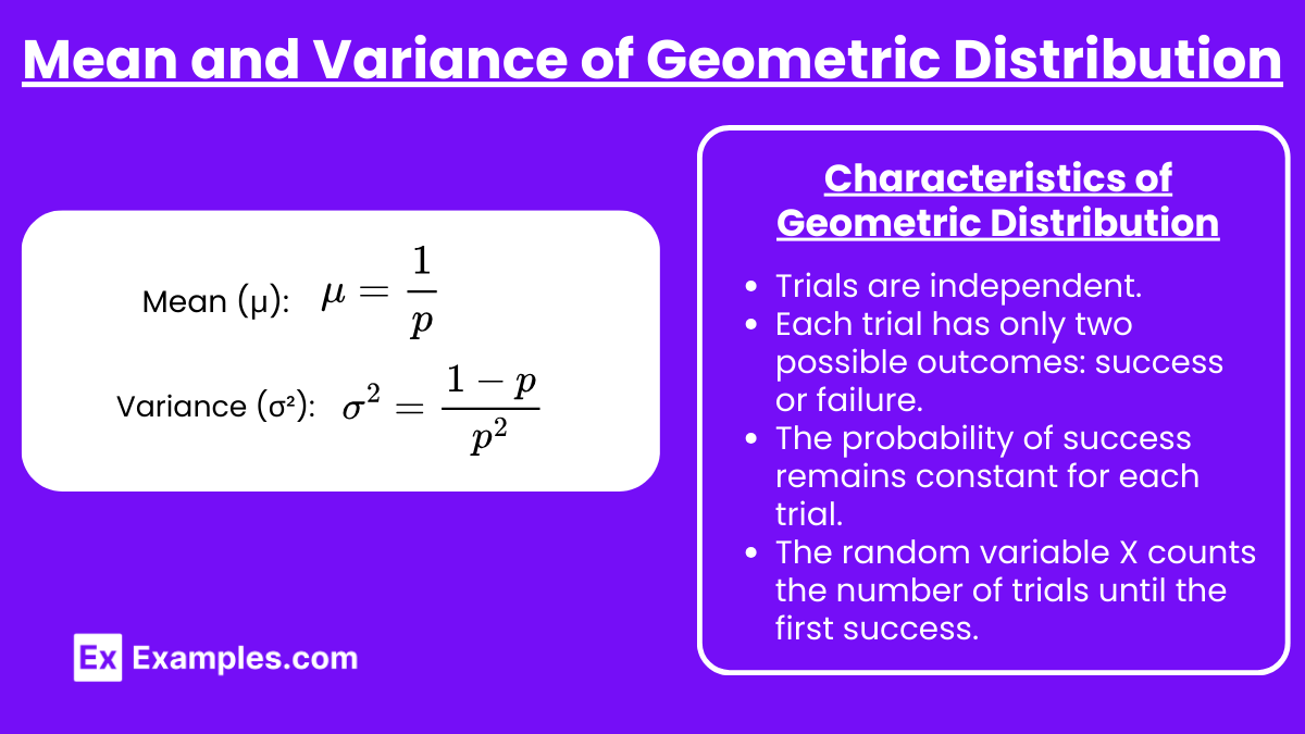
Mean (μ):
Variance (σ²):
Characteristics of Geometric Distribution
Trials are independent.
Each trial has only two possible outcomes: success or failure.
The probability of success remains constant for each trial.
The random variable X counts the number of trials until the first success.
Examples
Example 1: Coin Tossing
What is the probability that the first head appears on the 4th toss of a fair coin?
$
\begin{aligned}
p &= 0.5 \
k &= 4 \
P(X = 4) &= (1 - 0.5)^{4 - 1} \times 0.5 = (0.5)^3 \times 0.5 = 0.0625
\end{aligned}
$
Example 2: Quality Control
A factory produces items with a 5% defect rate. What is the probability that the first defect is found on the 3rd item inspected?
$
\begin{aligned}
p &= 0.05 \
k &= 3 \
P(X = 3) &= (1 - 0.05)^{3 - 1} \times 0.05 = (0.95)^2 \times 0.05 \approx 0.0451
\end{aligned}
$
Example 3: Basketball Free Throws
A basketball player has a 70% chance of making a free throw. What is the probability that the first made free throw happens on the 2nd attempt?
$
\begin{aligned}
p &= 0.7 \
k &= 2 \
P(X = 2) &= (1 - 0.7)^{2 - 1} \times 0.7 = (0.3)^1 \times 0.7 = 0.21
\end{aligned}
$
Example 4: Dice Rolling
If a die is rolled, what is the probability that the first 6 appears on the 5th roll?
$
\begin{aligned}
p &= \frac{1}{6} \
k &= 5 \
P(X = 5) &= \left(1 - \frac{1}{6}\right)^{5 - 1} \times \frac{1}{6} = \left(\frac{5}{6}\right)^4 \times \frac{1}{6} \approx 0.0804
\end{aligned}
$
Example 5: Customer Service Calls
A customer service center answers calls with a 15% chance of solving a customer's problem on the first attempt. What is the probability that the first successful resolution occurs on the 6th call?
$
\begin{aligned}
p &= 0.15 \
k &= 6 \
P(X = 6) &= (1 - 0.15)^{6 - 1} \times 0.15 = (0.85)^5 \times 0.15 \approx 0.0770
\end{aligned}
$
Multiple Choice Questions (MCQs)
MCQ 1
A die is rolled, and the probability of rolling a 4 is . What is the probability that the first 4 appears on the 3rd roll?
A. 0.0462
B. 0.1157
C. 0.0972
D. 0.1986
Answer: A
Explanation:
$
\begin{aligned}
p &= \frac{1}{6} \
k &= 3 \
P(X = 3) &= \left(1 - \frac{1}{6}\right)^{3 - 1} \times \frac{1}{6} = \left(\frac{5}{6}\right)^2 \times \frac{1}{6} \approx 0.0462
\end{aligned}
$
MCQ 2
A student has a 30% chance of guessing the correct answer on a multiple-choice question. What is the probability that the first correct answer is on the 4th guess?
A. 0.0729
B. 0.1029
C. 0.0459
D. 0.0891
Answer: B
Explanation:
$
\begin{aligned}
p &= 0.3 \
k &= 4 \
P(X = 4) &= (1 - 0.3)^{4 - 1} \times 0.3 = (0.7)^3 \times 0.3 = 0.1029
\end{aligned}
$
MCQ 3
In a factory, the probability of producing a defective item is 0.1. What is the probability that the first defective item is produced on the 5th try?
A. 0.0656
B. 0.0737
C. 0.0810
D. 0.0914
Answer: C
Explanation:
$
\begin{aligned}
p &= 0.1 \
k &= 5 \
P(X = 5) &= (1 - 0.1)^{5 - 1} \times 0.1 = (0.9)^4 \times 0.1 = 0.0656
\end{aligned}
$