Excel Formulas list with Examples

Excel formulas are powerful tools that enhance data analysis and manipulation capabilities within Microsoft Excel, particularly for inventory control and managing agenda. They allow users to perform a wide range of calculations, from simple arithmetic to complex statistical analysis. Common Excel formulas include SUM, AVERAGE, VLOOKUP, and IF, each serving different purposes to streamline workflows and improve productivity. By mastering these formulas, users can efficiently manage large datasets, automate repetitive tasks, and gain deeper insights into their inventory control processes and agendas. This guide provides a comprehensive list of Excel formulas with practical examples..

What is Excel Formula? 

An Excel formula is a combination of cell references, operators, and functions used to perform calculations or logical operations. Formulas start with an equals sign (=) and can include mathematical operations, text manipulation, and more, enhancing data analysis and spreadsheet functionality.

Excel Formulas List with Examples

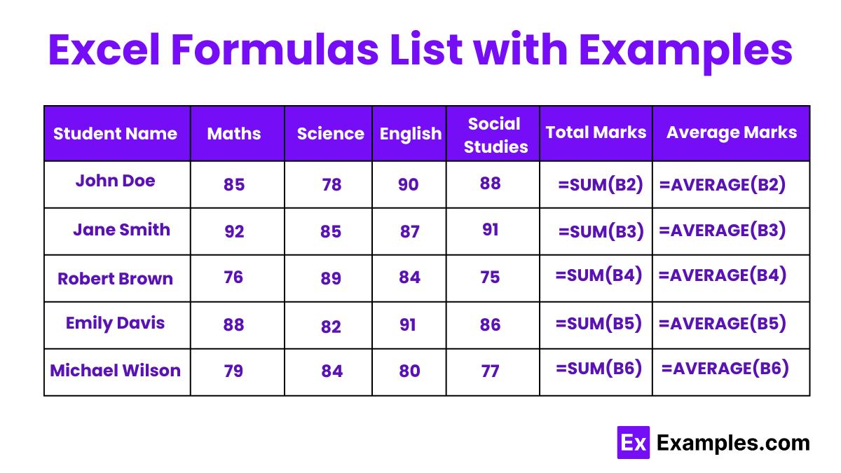
1. SUM

Formula: =SUM(A1:A10)
Example: Adds all numbers in cells A1 through A10.

2. AVERAGE

Formula: =AVERAGE(B1:B10)
Example: Calculates the average of the numbers in cells B1 through B10.

3. VLOOKUP

Formula: =VLOOKUP(lookup_value, table_array, col_index_num, [range_lookup])
Example: =VLOOKUP(A2, $B$2:$D$10, 3, FALSE)
Looks for the value in cell A2 in the first column of the range B2:D10 and returns the value in the third column of the range.

4. IF

Formula: =IF(logical_test, value_if_true, value_if_false)
Example: =IF(C2>50, "Pass", "Fail")
Checks if the value in cell C2 is greater than 50, returns “Pass” if true, and “Fail” if false.

5. CONCATENATE (or CONCAT)

Formula: =CONCATENATE(text1, [text2], ...)
Example: =CONCATENATE(A2, " ", B2)
Combines the text in cells A2 and B2 with a space in between.

6. MAX

Formula: =MAX(D1:D10)
Example: Returns the largest number in the range D1 to D10.

7. MIN

Formula: =MIN(E1:E10)
Example: Returns the smallest number in the range E1 to E10.

8. COUNT

Formula: =COUNT(F1:F10)
Example: Counts the number of numeric entries in the range F1 to F10.

9. COUNTA

Formula: =COUNTA(G1:G10)
Example: Counts the number of non-empty cells in the range G1 to G10.

10. LEN

Formula: =LEN(text)
Example: =LEN(H1)
Returns the number of characters in cell H1.

11. TRIM

Formula: =TRIM(text)
Example: =TRIM(I1)
Removes extra spaces from the text in cell I1.

12. ROUND

Formula: =ROUND(number, num_digits)
Example: =ROUND(J1, 2)
Rounds the number in cell J1 to two decimal places.

13. LEFT

Formula: =LEFT(text, [num_chars])
Example: =LEFT(K1, 3)
Returns the first three characters from the text in cell K1.

14. RIGHT

Formula: =RIGHT(text, [num_chars])
Example: =RIGHT(L1, 4)
Returns the last four characters from the text in cell L1.

15. MID

Formula: =MID(text, start_num, num_chars)
Example: =MID(M1, 2, 5)
Returns five characters from the text in cell M1, starting from the second character.

16. NOW

Formula: =NOW()
Example: Returns the current date and time.

17. TODAY

Formula: =TODAY()
Example: Returns the current date.

18. DATE

Formula: =DATE(year, month, day)
Example: =DATE(2023, 6, 12)
Returns the date June 12, 2023.

19. DATEDIF

Formula: =DATEDIF(start_date, end_date, unit)
Example: =DATEDIF(A1, B1, "D")
Returns the number of days between the dates in cells A1 and B1.

20. SUMIF

Formula: =SUMIF(range, criteria, [sum_range])
Example: =SUMIF(N1:N10, ">100", O1:O10)
Adds the numbers in the range O1:O10 where the corresponding cells in N1:N10 are greater than 100.

21. COUNTIF

Formula: =COUNTIF(range, criteria)
Example: =COUNTIF(P1:P10, "Apples")
Counts the number of cells in the range P1:P10 that contain the word “Apples”.

22. AVERAGEIF

Formula: =AVERAGEIF(range, criteria, [average_range])
Example: =AVERAGEIF(Q1:Q10, ">=70", R1:R10)
Calculates the average of the numbers in the range R1:R10 where the corresponding cells in Q1:Q10 are greater than or equal to 70.

23. ABS

Formula: =ABS(number)
Example: =ABS(S1)
Returns the absolute value of the number in cell S1.

24. SQRT

Formula: =SQRT(number)
Example: =SQRT(T1)
Returns the square root of the number in cell T1.

25. POWER

Formula: =POWER(number, power)
Example: =POWER(U1, 3)
Returns the value of the number in cell U1 raised to the power of 3.

26. SUMPRODUCT

Formula: =SUMPRODUCT(array1, [array2], ...)
Example: =SUMPRODUCT(V1:V10, W1:W10)
Returns the sum of the products of corresponding ranges or arrays V1:V10 and W1:W10.

27. INDEX

Formula: =INDEX(array, row_num, [column_num])
Example: =INDEX(X1:Y10, 3, 2)
Returns the value in the third row and second column of the range X1:Y10.

28. MATCH

Formula: =MATCH(lookup_value, lookup_array, [match_type])
Example: =MATCH(A2, Z1:Z10, 0)
Returns the relative position of the value in cell A2 within the range Z1:Z10.

29. INDIRECT

Formula: =INDIRECT(ref_text, [a1])
Example: =INDIRECT("A" & B1)
Returns the reference specified by a text string, combining “A” with the value in cell B1.

30. CHOOSE

Formula: =CHOOSE(index_num, value1, [value2], ...)
Example: =CHOOSE(2, "Red", "Blue", "Green")
Returns “Blue” because it is the second value in the list.

31. ISBLANK

Formula: =ISBLANK(value)
Example: =ISBLANK(C1)
Returns TRUE if cell C1 is empty.

32. ISNUMBER

Formula: =ISNUMBER(value)
Example: =ISNUMBER(D1)
Returns TRUE if cell D1 contains a number.

33. ISERROR

Formula: =ISERROR(value)
Example: =ISERROR(E1)
Returns TRUE if cell E1 contains an error.

34. AND

Formula: =AND(logical1, [logical2], ...)
Example: =AND(F1>10, G1<5)
Returns TRUE if both conditions are true.

35. OR

Formula: =OR(logical1, [logical2], ...)
Example: =OR(H1="Yes", I1="No")
Returns TRUE if either condition is true.

36. NOT

Formula: =NOT(logical)
Example: =NOT(J1>10)
Returns TRUE if the condition is false.

37. TRUE

Formula: =TRUE()
Example: Returns the logical value TRUE.

38. FALSE

Formula: =FALSE()
Example: Returns the logical value FALSE.

39. IFERROR

Formula: =IFERROR(value, value_if_error)
Example: =IFERROR(A1/B1, "Error")
Returns “Error” if the division of A1 by B1 results in an error.

40. RANK

Formula: =RANK(number, ref, [order])
Example: =RANK(K1, L1:L10)
Returns the rank of a number in a list of numbers.

41. TRANSPOSE

Formula: =TRANSPOSE(array)
Example: =TRANSPOSE(M1:O3)
Converts a vertical range of cells to a horizontal range, or vice versa.

42. UNIQUE

Formula: =UNIQUE(array)
Example: =UNIQUE(P1:P10)
Returns the unique values in the range P1:P10.

43. FILTER

Formula: =FILTER(array, include, [if_empty])
Example: =FILTER(Q1:Q10, R1:R10>50)
Returns an array

of values from Q1:Q10 where the corresponding values in R1:R10 are greater than 50.

44. SORT

Formula: =SORT(array, [sort_index], [sort_order])
Example: =SORT(S1:S10, 1, 1)
Sorts the range S1:S10 in ascending order.

45. SEQUENCE

Formula: =SEQUENCE(rows, [columns], [start], [step])
Example: =SEQUENCE(5, 1, 1, 1)
Generates a sequence of numbers from 1 to 5 in a single column.

46. SUMSQ

Formula: =SUMSQ(number1, [number2], ...)
Example: =SUMSQ(T1:T5)
Returns the sum of the squares of the numbers in the range T1:T5.

47. PRODUCT

Formula: =PRODUCT(number1, [number2], ...)
Example: =PRODUCT(U1:U5)
Returns the product of the numbers in the range U1:U5.

48. FACT

Formula: =FACT(number)
Example: =FACT(5)
Returns the factorial of 5 (5!).

49. PI

Formula: =PI()
Example: Returns the value of π (3.14159…).

50. MOD

Formula: =MOD(number, divisor)
Example: =MOD(V1, 3)
Returns the remainder of the division of the number in cell V1 by 3.

51. LARGE

Formula: =LARGE(array, k)
Example: =LARGE(W1:W10, 2)
Returns the second largest value in the range W1:W10.

52. SMALL

Formula: =SMALL(array, k)
Example: =SMALL(X1:X10, 3)
Returns the third smallest value in the range X1:X10.

53. FORECAST

Formula: =FORECAST(x, known_y's, known_x's)
Example: =FORECAST(10, Y1:Y10, Z1:Z10)
Returns a predicted value based on the linear trend of the known data.

54. HLOOKUP

Formula: =HLOOKUP(lookup_value, table_array, row_index_num, [range_lookup])
Example: =HLOOKUP(A1, B1:D10, 3, FALSE)
Looks for the value in cell A1 in the first row of the range B1:D10 and returns the value in the third row of the range.

55. OFFSET

Formula: =OFFSET(reference, rows, cols, [height], [width])
Example: =OFFSET(A1, 2, 3)
Returns the value of the cell that is 2 rows down and 3 columns to the right of cell A1.

56. TEXT

Formula: =TEXT(value, format_text)
Example: =TEXT(B1, "0.00")
Formats the number in cell B1 to have two decimal places.

57. VALUE

Formula: =VALUE(text)
Example: =VALUE("123.45")
Converts the text string “123.45” to the number 123.45.

58. FIND

Formula: =FIND(find_text, within_text, [start_num])
Example: =FIND("apple", C1)
Returns the position of the first occurrence of “apple” in cell C1.

59. SEARCH

Formula: =SEARCH(find_text, within_text, [start_num])
Example: =SEARCH("dog", D1)
Returns the position of the first occurrence of “dog” in cell D1, case-insensitive.

60. REPLACE

Formula: =REPLACE(old_text, start_num, num_chars, new_text)
Example: =REPLACE(E1, 1, 3, "cat")
Replaces the first three characters of the text in cell E1 with “cat”.

61. SUBSTITUTE

Formula: =SUBSTITUTE(text, old_text, new_text, [instance_num])
Example: =SUBSTITUTE(F1, "red", "blue")
Replaces all occurrences of “red” with “blue” in cell F1.

Excel Formulas and Functions

Basic Arithmetic Functions

SUM is the most basic and widely used function in Excel, allowing users to add values across a range of cells, which is especially useful for payment calculations. For example, =SUM(A1:A10) sums all payment amounts in cells A1 through A10. Similarly, AVERAGE calculates the mean of a range of values, such as =AVERAGE(B1:B10), providing a quick way to determine the average payment amount in a dataset.

Lookup and Reference Functions

Functions like VLOOKUP and HLOOKUP are essential for searching for a value in a table and returning data from a specific column or row. For instance, =VLOOKUP(A2, $B$2:$D$10, 3, FALSE) looks up the value in cell A2 within the range B2:D10 and returns the corresponding value from the third column. The INDEX and MATCH functions are also powerful for more complex lookups. =INDEX(X1:Y10, 3, 2) retrieves the value in the third row and second column of the specified range.

Logical Functions

Logical functions help users make decisions based on certain conditions. The IF function, =IF(C2>50, "Pass", "Fail"), evaluates whether a condition is true or false and returns one value if true and another if false. Combined with AND and OR functions, users can build more complex logical tests, such as =AND(F1>10, G1<5) and =OR(H1="Yes", I1="No").

Text Functions

Text functions are useful for manipulating and combining text strings. CONCATENATE (or the newer CONCAT function), =CONCATENATE(A2, " ", B2), merges text from multiple cells into one. LEFT, RIGHT, and MID functions extract specific portions of a text string, while TRIM removes unnecessary spaces. For example, =LEFT(K1, 3) extracts the first three characters from a text string in cell K1.

Date and Time Functions

Excel also includes functions to handle dates and times efficiently, which is essential for employee tracking. The TODAY function, =TODAY(), returns the current date, while NOW, =NOW(), gives the current date and time. Functions like DATEDIF, =DATEDIF(A1, B1, “D”), calculate the difference between two dates, making it useful for tracking employee age or tenure.

Statistical Functions

For statistical analysis, functions like MAX, =MAX(D1:D10), and MIN, =MIN(E1:E10), quickly find the largest and smallest values in a range. The COUNT function, =COUNT(F1:F10), counts the number of numeric entries, while COUNTA counts all non-empty cells.

Array Functions

Array functions, such as SUMPRODUCT, =SUMPRODUCT(V1:V10, W1:W10), multiply corresponding elements in given arrays and return the sum of those products. The TRANSPOSE function, =TRANSPOSE(M1:O3), converts a vertical range of cells to a horizontal range, or vice versa, facilitating data manipulation.

Error Handling Functions

To manage errors in formulas, IFERROR provides a way to catch and handle errors gracefully. For example, =IFERROR(A1/B1, "Error") returns “Error” if the division operation results in an error, preventing the display of unsightly error messages.

Financial and Mathematical Functions

Excel also offers a range of financial and mathematical functions. ABS returns the absolute value of a number, while POWER raises a number to a specified power. RANK provides the rank of a number within a list, and ROUND helps in rounding numbers to a specified number of digits.

By mastering these Excel formulas and functions, users can significantly enhance their data processing capabilities, making complex analyses more straightforward and efficient. Whether for basic arithmetic, complex lookups, logical tests, or statistical analysis, Excel’s vast array of functions caters to a wide range of data manipulation needs.

Why Are Excel Formulas Important?

1. Efficiency and Time-Saving : Excel formulas automate calculations and data processing tasks that would otherwise be time-consuming and prone to errors if done manually. By using formulas like SUM, AVERAGE, and COUNT, users can quickly compute totals, averages, and counts across large datasets, saving significant time and effort.

2. Accuracy : Formulas ensure consistency and accuracy in calculations, which is crucial when working with qualitative data. Once a formula is correctly set up, it eliminates the risk of human error in repetitive calculations. For example, using the IF function for logical tests or VLOOKUP for data retrieval ensures that the results are accurate and reliable when analyzing qualitative data.

3. Data Analysis and Insights : Excel formulas facilitate in-depth data analysis, allowing users to extract meaningful insights from raw data. Functions such as MAX, MIN, and AVERAGE help identify trends, outliers, and key metrics. Pivot tables and advanced formulas like INDEX and MATCH enable complex data manipulation and analysis.

4. Automation : Formulas can automate repetitive tasks, reducing the need for manual intervention. For instance, using conditional formatting with logical formulas can automatically highlight cells that meet specific criteria. Similarly, array functions like SUMPRODUCT can perform multiple calculations on arrays of data in one go.

5. Dynamic Data Updates : Formulas ensure that data updates dynamically. When input values change, the formulas recalculate automatically, providing up-to-date results without the need for manual recalculations. This is particularly useful for financial modeling, budgeting, and forecasting.

6. Simplified Data Management : With functions like CONCATENATE (or CONCAT), LEFT, RIGHT, and MID, Excel makes it easy to manage and manipulate text data. This is essential for cleaning data, combining information from multiple sources, and preparing datasets for analysis.

7. Enhanced Reporting : Formulas enhance the quality and clarity of payroll sheets. By using functions like SUMIF, COUNTIF, and AVERAGEIF, users can create detailed and specific summaries of data. This makes it easier to generate payroll sheets that are both comprehensive and easy to understand.

8. Decision Making : Excel formulas support informed decision-making by providing clear and precise data analysis for budget plans. Logical functions like IF, AND, OR, and NOT help in setting up decision-making frameworks within spreadsheets. This ensures that budget plans are based on accurate and current data.

9. Versatility : Excel formulas are versatile and can be used across various fields and industries, including finance, marketing, sales, engineering, and research. Their wide applicability makes them a valuable tool for professionals in different sectors.

10. Learning and Development : Understanding and using Excel formulas can significantly enhance one’s data analysis and problem-solving skills. It also improves proficiency in Excel, which is a valuable skill in the job market.

Five Time-saving Ways to Insert Data into Excel

1. Copy and Paste : Copying and pasting data is one of the simplest and most commonly used methods to transfer data into Excel. You can copy data from other spreadsheets, web pages, or documents and paste it directly into Excel cells. Use Ctrl+C to copy and Ctrl+V to paste. For pasting values only, use Ctrl+Shift+V. This method is quick and effective for transferring large amounts of data without retyping.

2. Flash Fill : Flash Fill is a powerful feature that automatically fills your data when it detects a pattern. For example, if you have a list of names in column A and you want to separate first and last names into columns B and C, start typing the first name in column B. Excel will recognize the pattern and suggest the remaining names. Simply press Enter to accept the suggestions. This tool can save a significant amount of time with repetitive data entry tasks.

3. AutoFill : AutoFill allows you to quickly fill cells with repetitive or sequential data. Click and drag the fill handle (a small square at the bottom-right corner of the selected cell) to copy the cell’s content or extend a series (e.g., dates, numbers, or custom lists). For instance, entering “Monday” and dragging the fill handle will automatically fill the cells with the subsequent days of the week. This method is excellent for speeding up the entry of recurring or patterned data.

4. Import Data from External Sources : Excel supports importing data from various external sources such as text files, CSV files, databases, and web pages. Use the “Get Data” feature under the “Data” tab to import data. This method is particularly useful for large datasets, as it eliminates the need for manual entry. Additionally, you can refresh the data connections to keep your spreadsheet updated with the latest information from the source.

5. Use Excel Forms : Excel Forms provide a user-friendly way to enter data into a table format. Activate the Form tool by adding it to the Quick Access Toolbar. Once set up, the form interface allows you to input data into fields, navigate through records, and quickly add new entries. This method simplifies data entry, especially for users unfamiliar with Excel’s grid format, and ensures that data is consistently and accurately entered into the correct columns.

How to Use Excel Formulas

1. Understanding the Basics of Formulas : Excel formulas always start with an equals sign (=). This tells Excel that the following string of characters constitutes a formula. Formulas can perform a variety of operations, from simple arithmetic to complex statistical analysis. For example, =A1 + B1 adds the values in cells A1 and B1. Understanding this basic structure is the first step in mastering Excel formulas.

2. Using Built-in Functions : Excel provides numerous built-in functions that can simplify complex calculations. Functions like SUM, AVERAGE, and VLOOKUP are powerful tools for aggregating and analyzing data. To use a function, type the equals sign followed by the function name and arguments in parentheses. For instance, =SUM(A1:A10) adds all the numbers in the range A1 to A10. Familiarize yourself with Excel’s function library to leverage these tools effectively.

3. Combining Functions and Operators : You can combine multiple functions and arithmetic operators to create more complex formulas. For example, =SUM(A1:A10) / COUNT(A1:A10) calculates the average value of a range by dividing the sum by the count. Understanding how to nest functions within each other and use operators like +, -, *, and / allows you to perform sophisticated calculations.

4. Referencing Cells and Ranges : Excel formulas often reference other cells or ranges to retrieve data. Absolute references (using $) and relative references are crucial concepts. An absolute reference, like $A$1, keeps the same cell reference even when the formula is copied to another cell. A relative reference, like A1, adjusts based on the position of the formula. Knowing when to use each type helps maintain accuracy in your calculations.

5. Applying Formulas to Multiple Cells : You can apply a formula to multiple cells using the fill handle. After typing your formula, click and drag the fill handle (a small square at the bottom-right corner of the selected cell) to copy the formula across adjacent cells. This technique is useful for applying the same calculation across a dataset, saving time and ensuring consistency.

6. Error Checking and Troubleshooting : Excel provides tools to help you check for and fix errors in your formulas. Common errors include #DIV/0! (division by zero) and #N/A (value not available). Use the IFERROR function to handle errors gracefully. For instance, =IFERROR(A1/B1, "Error") returns “Error” if there’s a division by zero. Additionally, the Formula Auditing toolbar can help trace precedents and dependents, making it easier to troubleshoot issues.

7. Utilizing Named Ranges : Named ranges are a way to simplify formulas and make them easier to understand. Instead of using cell references, you can assign a name to a range of cells and use that name in your formulas. For example, if you name the range A1:A10 as “Sales”, you can use =SUM(Sales) instead of =SUM(A1:A10). This practice improves formula readability and reduces errors.

8. Exploring Advanced Functions : Excel’s advanced functions, such as INDEX, MATCH, ARRAYFORMULA, and OFFSET, provide powerful capabilities for dynamic and complex calculations. These functions allow for more sophisticated data manipulation and analysis. For instance, =INDEX(B2:D10, MATCH("Product", A2:A10, 0), 2) can look up and return data from a specific row and column. Learning these advanced functions can significantly enhance your data analysis skills.

Best practices for writing Excel formulas

Writing Excel formulas effectively can significantly enhance your productivity and ensure the accuracy of your data analysis. Here are some best practices to follow:

1. Use Descriptive Naming Conventions : When naming cells or ranges, use descriptive names that reflect the data they contain. Instead of using generic names like Range1, use Sales Data or Total Expenses. This practice makes your formulas easier to understand and maintain. For example, =SUM (Sales Data) is much clearer than =SUM(A1:A10).

2. Keep Formulas Simple : Complex formulas can be difficult to read and troubleshoot. Break down complex calculations into simpler steps and use intermediate cells to hold partial results. This not only makes your formulas more understandable but also easier to debug. For instance, instead of writing =SUM(A1:A10)/COUNT(A1:A10), you can calculate SUM(A1:A10) in one cell and COUNT(A1:A10) in another, then divide the two results in a third cell.

3. Use Absolute and Relative References Appropriately : Understand when to use absolute references ($A$1) versus relative references (A1). Absolute references remain constant when copying formulas, while relative references adjust based on their position. Use absolute references for fixed values and relative references for dynamic ranges. For example, =A1*$B$1 keeps the reference to cell B1 constant, even if the formula is copied to other cells.

4. Document Your Formulas : Add comments to your formulas to explain their purpose and logic. While Excel itself does not support inline comments within formulas, you can use cell comments or a separate documentation sheet. Documenting your formulas helps others (and yourself) understand the rationale behind complex calculations, especially when revisiting the spreadsheet after some time.

5. Test and Validate Formulas : Before finalizing your formulas, test them with different data sets to ensure they work correctly under various scenarios. Validate your results by comparing them with known outcomes or using manual calculations. This practice helps identify and correct errors early, ensuring the reliability of your analysis.

6. Use Built-in Functions : Excel offers a wide range of built-in functions that can simplify your formulas. Instead of creating complex nested formulas, leverage these functions to perform common tasks. For example, use SUMIF and COUNTIF for conditional sums and counts, rather than combining SUM and IF functions manually. This not only reduces formula complexity but also enhances performance.

7. Handle Errors Gracefully : Use error-handling functions like IFERROR to manage potential errors in your formulas. For example, =IFERROR(A1/B1, "Error") returns “Error” if there is a division by zero, preventing Excel from displaying an error message. Handling errors gracefully ensures your spreadsheet remains functional and user-friendly, even when unexpected data issues occur.

8. Keep Formulas Consistent : Maintain consistency in your formulas to avoid confusion and errors. Use similar structures and logic throughout your spreadsheet, especially when performing the same types of calculations. Consistent formulas are easier to understand and maintain, reducing the likelihood of mistakes.

9. Optimize Performance : Large and complex formulas can slow down your spreadsheet. Optimize performance by minimizing the use of volatile functions (like NOW and RAND), which recalculate every time the sheet changes. Use efficient formulas and limit the number of calculations in large datasets. For example, use SUMPRODUCT instead of array formulas, which are typically faster and more efficient.

10. Protect Your Formulas : To prevent accidental changes, protect your formulas by locking the cells containing them. Go to the Review tab, click on Protect Sheet, and select the appropriate options. This practice ensures the integrity of your formulas, especially in shared workbooks where multiple users have access.

Difference Between Formula and Functions in Excel

Aspect	Formula	Function
Definition	A combination of operators, cell references, and functions to perform calculations.	A predefined, named calculation provided by Excel to perform specific tasks.
Complexity	Can be simple or complex, depending on the combination of elements used.	Generally simpler as they are predefined and require specific arguments.
Customization	Can be customized extensively by combining various elements.	Limited to the predefined logic and arguments provided by Excel.
Examples	=A1 + B1 - C1	=SUM(A1:A10), =VLOOKUP(A1, B1:C10, 2, FALSE)
Use Cases	Used for both simple arithmetic operations and complex calculations involving multiple steps.	Used for specific tasks like summing a range, finding averages, or looking up values.
Syntax	General structure: =operand1 operator operand2 ...	Specific structure: =FUNCTION_NAME(argument1, argument2, ...)
Flexibility	Highly flexible, can include multiple functions and operators.	Less flexible, confined to the function’s specific purpose.
Error Handling	Errors can be complex to troubleshoot due to combinations of elements.	Errors are often easier to identify as they are related to specific functions.
Ease of Use	Can be more challenging to create and understand, especially complex formulas.	Easier to use for specific tasks, as they require knowledge of function arguments only.
Learning Curve	Requires understanding of operators, cell references, and potentially multiple functions.	Requires understanding of specific function syntax and arguments.