Curve-Based and Empirical Fixed-Income Risk Measures

Preparing for the CFA Exam involves a deep dive into “Curve-Based and Empirical Fixed-Income Risk Measures,” a key aspect of fixed-income analysis. Proficiency in understanding yield curves, spread measures, and empirical models is crucial. This knowledge helps in assessing risks and returns in the bond market, essential for a high CFA score.

Learning Objective

In studying “Curve-Based and Empirical Fixed-Income Risk Measures” for the CFA Exam, you should aim to understand key concepts related to assessing fixed-income risk, including yield curve shapes, shifts, and their implications on bond valuations. Analyze how curve-based measures, such as duration and convexity, help quantify interest rate sensitivity and risk exposure. Evaluate empirical risk models used in fixed-income analysis, focusing on factors like credit spreads, liquidity premiums, and term structure modeling. Additionally, explore the practical applications of these measures in portfolio management, and apply your knowledge to evaluate and mitigate risk in diverse bond portfolios, as emphasized in CFA practice scenarios.

Understanding Yield Curves and Interest Rate Risk

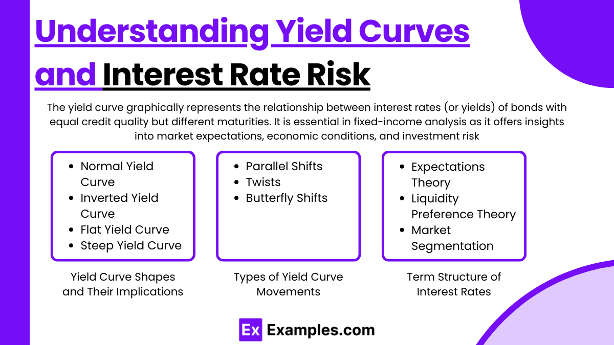
The yield curve is a graphical representation showing the relationship between interest rates (or yields) of bonds having equal credit quality but differing maturity dates. It is a critical tool in fixed-income analysis because it provides insights into market expectations, economic activity, and potential investment risk. Here’s an in-depth look at key aspects of yield curves and their role in assessing interest rate risk.

Yield Curve Shapes and Their Implications

1. Normal Yield Curve: Typically, a normal yield curve slopes upward, indicating that long-term interest rates are higher than short-term rates. This shape suggests that investors expect economic growth and possibly higher inflation in the future, which would require a premium for locking funds over a longer period.
2. Inverted Yield Curve: An inverted curve slopes downward, with short-term rates higher than long-term rates. This rare shape often signals an impending economic slowdown or recession, as investors expect future interest rates to fall.
3. Flat Yield Curve: A flat curve occurs when short-term and long-term rates are roughly equal. This shape usually suggests economic uncertainty or a transition period, where neither growth nor recession is imminent, and rates are expected to remain stable in the short term.
4. Steep Yield Curve: A steep curve, where long-term yields are significantly higher than short-term yields, often indicates strong economic growth expectations. Investors demand higher returns for longer maturities due to anticipated inflation and interest rate increases.

Types of Yield Curve Movements

Yield curves do not remain static; they can shift due to changes in market expectations and economic conditions. Key movements include:

1. Parallel Shifts: A parallel shift occurs when all points on the yield curve move up or down by the same magnitude. This movement implies that interest rates across all maturities have risen or fallen, usually due to a change in central bank policies or inflation expectations.
2. Twists: A twist happens when the yield curve pivots around a certain maturity point, causing short-term and long-term yields to move in opposite directions. A twist can reflect changing expectations for short-term versus long-term economic conditions or a shift in investor demand for different maturities.
3. Butterfly Shifts: A butterfly shift describes a scenario where the yield curve becomes more or less curved. For instance, the short- and long-term rates may rise while the medium-term rates remain stable or fall. This complex movement can indicate specific changes in investor preferences or economic expectations.

Term Structure of Interest Rates

The term structure of interest rates provides a theoretical framework to explain why yield curves take different shapes. Several theories attempt to explain the observed shape of the yield curve:

1. Expectations Theory: This theory posits that long-term rates are a reflection of expected future short-term rates. If investors expect rates to rise, the yield curve will slope upward; if they expect rates to fall, it will slope downward.
2. Liquidity Preference Theory: This theory suggests that investors demand a premium for holding longer-term securities due to the greater risk associated with time. This risk premium results in an upward-sloping curve, even if short-term rates are expected to stay constant.
3. Market Segmentation Theory: According to this theory, the bond market is divided into different segments based on maturity preferences of various investor groups. For example, pension funds may prefer long-term bonds, while corporations may prefer short-term ones. This preference structure shapes the yield curve independently of expected future rates.

Relevance of Yield Curves in Interest Rate Risk

Understanding the shape and movement of the yield curve is essential for managing interest rate risk. Interest rate risk reflects the potential change in bond prices due to fluctuations in market interest rates. Since bond prices and yields are inversely related, an increase in interest rates generally leads to a decrease in bond prices, and vice versa. By analyzing the yield curve, investors can gain insights into potential price volatility for different maturities and choose bonds that align with their risk tolerance and investment goals.

Duration and Convexity as Risk Measures

Duration and convexity are fundamental tools for assessing interest rate risk in fixed-income securities. These metrics help investors understand the sensitivity of bond prices to changes in interest rates, providing insights into how much a bond’s value may fluctuate with shifts in market rates. Here’s an in-depth look at duration and convexity and how they contribute to managing interest rate risk.

1. Duration: Measuring Sensitivity to Interest Rates

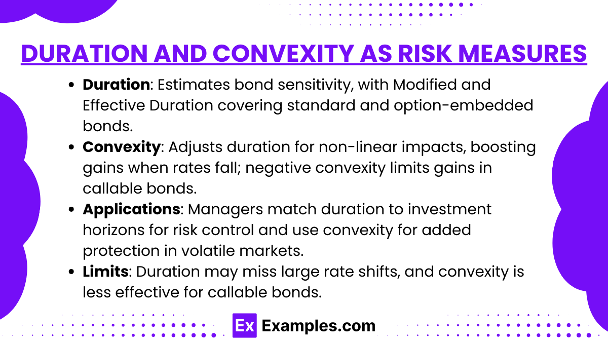
Duration is a measure of a bond’s sensitivity to changes in interest rates, reflecting the average time it takes to receive the bond’s cash flows, weighted by the present value of those cash flows. The higher the duration, the more sensitive a bond is to changes in interest rates. There are different types of duration, each suited to specific types of bonds and purposes:

• Macaulay Duration: This is the weighted average time to receive the bond’s cash flows. Originally developed to measure bond portfolios’ interest rate sensitivity, it indicates how long it takes, on average, to recoup the investment.
• Modified Duration: Modified duration is a variation of Macaulay duration that measures a bond’s price sensitivity to a 1% change in interest rates. It is a more practical measure for estimating bond price volatility since it directly reflects price changes with interest rate shifts.
• Effective Duration: For bonds with embedded options, like callable or putable bonds, modified duration isn’t as effective because the bond’s cash flows can change based on interest rates. Effective duration accounts for the potential impact of these embedded options on cash flows, making it a better measure for option-embedded bonds.Example: If a bond has a modified duration of 5, then a 1% increase in interest rates is expected to cause a 5% decrease in the bond’s price, and a 1% decrease in interest rates is expected to cause a 5% increase in the bond’s price.

2. Convexity: Refining the Duration Measure

Convexity is a measure that improves upon duration by accounting for the curvature in the price-yield relationship of bonds. While duration provides a linear approximation of how bond prices change with interest rates, convexity adjusts for the fact that this relationship is actually non-linear, especially for large changes in interest rates.

• Positive Convexity: Most traditional fixed-rate bonds exhibit positive convexity, meaning that the price-yield curve bends outward. Positive convexity implies that as interest rates decrease, the bond price rises at an increasing rate, and as rates increase, the bond price falls at a decreasing rate. This characteristic benefits the investor in volatile interest rate environments, as the price gains are larger when rates drop than the losses when rates rise.
• Negative Convexity: Certain bonds, like callable bonds, exhibit negative convexity when interest rates fall to a level where the bond is likely to be called. In these cases, the bond’s price does not increase as much as would be expected from a bond with positive convexity, limiting the upside potential.Example: A bond with high convexity will gain more in price when interest rates drop and lose less when interest rates rise, compared to a bond with low convexity. This makes convexity particularly valuable for measuring risk in bonds with long maturities or embedded options.

3. Practical Application of Duration and Convexity in Portfolio Management

Duration and convexity are essential for managing interest rate risk in bond portfolios. By understanding both measures, portfolio managers can tailor their strategies to align with their interest rate forecasts and risk tolerance. Here’s how they are applied:

• Matching Duration with Investment Horizon: Portfolio managers may use duration to match the investment horizon with the bond’s duration, aiming to minimize interest rate risk. This approach, known as immunization, protects against interest rate fluctuations over the holding period.
• Adjusting for Interest Rate Volatility: Convexity becomes crucial when managers anticipate significant interest rate movements. High convexity bonds are more resilient to interest rate changes and are preferred in volatile markets, as they offer better protection against losses.

4. Limitations of Duration and Convexity

While duration and convexity provide valuable insights, they are not foolproof measures:

• Duration’s Linear Approximation: Duration only offers a linear estimate, which may not accurately predict price changes for significant interest rate shifts. Convexity helps to adjust for this but may still be limited for complex bonds with changing cash flows.
• Convexity and Callable Bonds: Convexity can be less reliable for callable bonds since the potential for early redemption affects price behavior differently

Credit Spreads and Liquidity Premiums

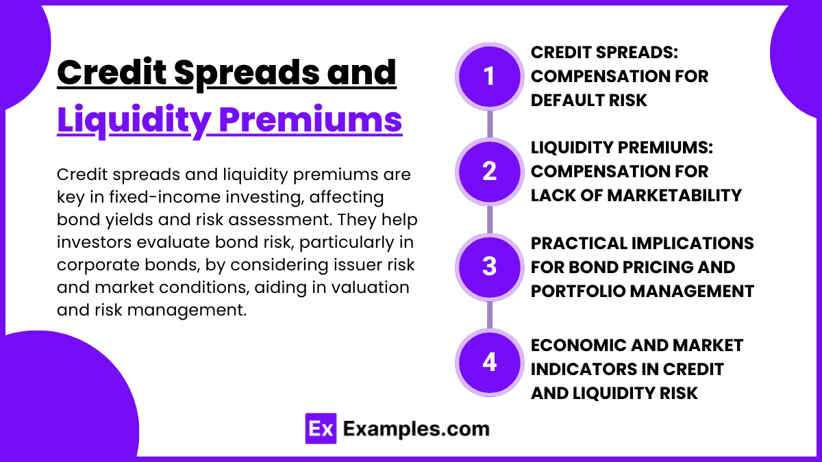
Credit spreads and liquidity premiums are critical elements in fixed-income investing, impacting bond yields and risk assessments. Understanding these factors helps investors evaluate a bond’s risk level, particularly in corporate and other non-government bonds, where issuer risk and market conditions play significant roles. Here’s an in-depth look at credit spreads, liquidity premiums, and their implications for bond valuation and risk management.

1. Credit Spreads: Compensation for Default Risk

A credit spread is the difference in yield between a corporate bond and a government bond of the same maturity. This spread represents the extra yield investors require for taking on the additional risk associated with corporate issuers, especially the risk of default. Credit spreads vary by credit rating, economic conditions, and investor sentiment, serving as a barometer for credit risk in the market.

• Credit Spread and Credit Ratings: Bonds are rated by credit rating agencies (e.g., Moody’s, S&P, Fitch), which assign ratings based on the issuer’s creditworthiness. Higher-rated bonds (e.g., AAA) have lower credit spreads, while lower-rated or high-yield (junk) bonds have wider spreads to compensate for greater default risk.Example: A AAA-rated corporate bond may have a credit spread of 0.5% over a comparable U.S. Treasury bond, while a BB-rated bond may have a spread of 3%, reflecting the additional risk investors take on with lower-rated bonds.
• Economic Influence on Credit Spreads: Credit spreads widen during economic downturns as default risk increases and narrow during economic growth when issuers are less likely to default. Thus, credit spreads are closely tied to the economic cycle and can signal market sentiment about credit risk.
• Yield Spread Curve: The shape of the yield spread curve, or credit spread curve, reflects market perceptions of credit risk across different maturities. In a stable market, the curve typically slopes upward, meaning longer-term bonds have higher spreads due to greater uncertainty. In times of high economic stress, the curve can flatten or invert.

2. Liquidity Premiums: Compensation for Lack of Marketability

Liquidity premium is the additional yield investors demand for bonds that are less easily traded or may have fewer buyers in the market. A liquidity premium compensates investors for the potential difficulty in selling a bond without impacting its price.

• Marketability and Trading Volume: Bonds with high trading volumes, like U.S. Treasuries, have minimal or no liquidity premium because they are highly liquid. Conversely, corporate bonds, especially those of smaller issuers or lower credit ratings, typically require a liquidity premium because they may be harder to sell in secondary markets.Example: A small-issuer corporate bond may trade with a 0.5% liquidity premium, reflecting the higher yield required by investors to hold a less liquid asset.
• Impact of Liquidity Conditions on Bond Yields: In times of market stress or economic instability, liquidity premiums rise as investors prefer more liquid assets and become reluctant to hold illiquid bonds. This dynamic can lead to a wider spread between liquid government securities and less liquid corporate bonds.
• Liquidity Premium and Maturity: Liquidity premiums are generally more pronounced for longer-maturity bonds due to increased uncertainty about the bond’s marketability over a more extended period. Short-term bonds usually have lower liquidity premiums because they mature faster, reducing exposure to liquidity risks.

3. Practical Implications for Bond Pricing and Portfolio Management

Credit spreads and liquidity premiums directly affect bond pricing and portfolio management strategies, as they provide insights into the underlying risk and yield compensation.

• Credit Spread Analysis for Portfolio Construction: Portfolio managers assess credit spreads to choose bonds that offer an attractive balance of risk and return. Wider credit spreads provide higher yields but also reflect higher risk, making them suitable for risk-tolerant investors. Narrow credit spreads, seen in higher-rated bonds, offer lower yields and lower risk, aligning with more conservative portfolios.
• Liquidity Premiums and Bond Allocation: Liquidity preferences also play a role in portfolio construction. Investors in need of frequent liquidity may focus on highly liquid securities, even at the expense of yield. Conversely, long-term investors might be willing to accept liquidity premiums by holding less liquid bonds, given the higher yields as compensation.
• Stress Testing for Economic Scenarios: Credit spreads and liquidity premiums are dynamic and can shift with economic conditions. Portfolio managers often stress-test portfolios to evaluate how changes in credit spreads or liquidity conditions might affect bond prices. This approach allows them to anticipate and manage potential losses during economic downturns or periods of market illiquidity.

4. Economic and Market Indicators in Credit and Liquidity Risk

Credit spreads and liquidity premiums are also used as economic indicators:

• Credit Spreads as Economic Indicators: Widening credit spreads can indicate increasing economic uncertainty or deteriorating credit conditions, while narrowing spreads often signal economic stability or growth. Investors monitor spreads on corporate bonds, particularly high-yield bonds, for signs of changing economic risk.
• Liquidity Premiums and Market Sentiment: High liquidity premiums can reflect investor preference for safety and aversion to risk, often rising in times of economic crisis. In contrast, low liquidity premiums indicate greater market confidence and willingness to take on risk

Empirical Models for Fixed-Income Risk

Empirical models for fixed-income risk provide quantitative frameworks to assess interest rate and credit risk in bonds. These models use historical data and statistical techniques to identify patterns and risk factors affecting bond prices, enabling more accurate risk management and pricing. Here are key types:

1. Factor Models: Factor models break down bond risk into components like interest rates, credit spreads, and economic indicators. By identifying factors that drive yield and price changes, these models help in forecasting price volatility and managing risk across different market scenarios.
2. Principal Component Analysis (PCA): PCA is a statistical tool used to identify the main drivers of yield curve movements, isolating factors such as level, slope, and curvature. PCA helps in understanding how much of a bond’s price sensitivity is due to changes in these primary risk factors.
3. Term Structure Models: These models, like the Cox-Ingersoll-Ross and Vasicek models, describe how interest rates evolve over time. They allow for the valuation of fixed-income securities by modeling future rate changes, which is essential for assessing the risk in long-term bonds.

Empirical models are crucial for risk-adjusted bond pricing, portfolio construction, and stress testing, giving investors insight into how bond values respond to various economic and market conditions

Examples

Example 1

Parallel Shift in Yield Curve: In a parallel shift, all points on the yield curve move up or down by the same amount. For instance, if the yield curve experiences a 1% upward parallel shift, all bond yields across different maturities increase by 1%. This would lead to a decrease in bond prices, impacting fixed-income portfolios sensitive to interest rate changes.

Example 2

Duration Matching for Immunization: A portfolio manager holds a bond portfolio with an average duration of 5 years and aims to match it with an investment horizon to minimize interest rate risk. By adjusting the portfolio’s duration to match the time horizon, the manager seeks to “immunize” the portfolio, reducing the impact of interest rate changes on the portfolio’s value.

Example 3

Credit Spread Widening During Economic Downturns: During a recession, credit spreads on corporate bonds tend to widen due to increased default risk. For example, a BBB-rated corporate bond’s spread over a Treasury bond of the same maturity might widen from 1% to 2%. This wider spread reflects the higher yield required by investors to compensate for the increased risk of default.

Example 4

Using PCA for Yield Curve Analysis: A fixed-income analyst applies Principal Component Analysis (PCA) to decompose the yield curve into its main factors: level, slope, and curvature. The PCA reveals that 90% of yield curve variance can be attributed to changes in the overall level (e.g., parallel shifts), helping the analyst focus on this primary factor for risk management.

Example 5

Term Structure Model Application for Long-Term Bonds: A bond trader uses the Vasicek term structure model to evaluate a 10-year bond. The model provides insights into the future path of interest rates, allowing the trader to assess potential price changes in the bond under different interest rate scenarios. This helps the trader price the bond with a more accurate risk assessment

Practice Question

Question 1

Which of the following best describes the purpose of using duration in fixed-income risk measurement?

A) To measure the total return of a bond over its lifetime
B) To assess a bond’s sensitivity to changes in interest rates
C) To calculate the credit risk associated with a bond
D) To evaluate the liquidity premium of a bond

Answer: B) To assess a bond’s sensitivity to changes in interest rates

Explanation: Duration measures a bond’s sensitivity to interest rate changes, estimating how much the bond’s price will change for a 1% change in interest rates. It does not assess credit risk, liquidity premiums, or total return over the bond’s lifetime.

Question 2

Principal Component Analysis (PCA) is primarily used in yield curve analysis to:

A) Identify major factors affecting yield curve changes, such as level, slope, and curvature
B) Determine the exact price of a bond with embedded options
C) Predict the future default rates of corporate bonds
D) Calculate the tax implications of bond yield

Answer: A) Identify major factors affecting yield curve changes, such as level, slope, and curvature

Explanation: PCA is a statistical tool that helps identify primary factors like level, slope, and curvature that influence yield curve movements. It is not used to price bonds with options, predict default rates, or assess tax implications.

Question 3

If a fixed-income portfolio manager wants to minimize the impact of interest rate changes on a bond portfolio, which of the following strategies is most appropriate?

A) Holding bonds with the longest possible maturities
B) Increasing the portfolio’s convexity without regard to duration
C) Matching the portfolio’s duration with the investment horizon
D) Reducing the credit rating of bonds in the portfolio

Answer: C) Matching the portfolio’s duration with the investment horizon

Explanation: Duration matching, or immunization, involves aligning the portfolio’s duration with the investment horizon to minimize sensitivity to interest rate changes. This approach reduces interest rate risk, unlike options A, B, or D, which are less effective for managing interest rate sensitivity