Extensions of Multiple Regression

For CFA Level 2 candidates, mastering extensions of multiple regression is essential to address complex relationships and improve model accuracy in financial data analysis. These advanced techniques allow for a deeper exploration of variable interactions, non-linear relationships, and the handling of categorical variables, crucial in the Quantitative Methods section of the exam.

Learning Objective

In studying “Extensions of Multiple Regression” for the CFA exam, you should aim to gain an understanding of advanced regression techniques that enhance the flexibility and predictive power of basic multiple regression. This includes learning about interaction terms, polynomial regression, and dummy variables, as well as exploring how these techniques allow for more complex models that can better capture real-world financial relationships. You will also develop skills in identifying situations where these extensions are appropriate and gain the ability to interpret their results effectively in a financial context.

1. Interaction Terms

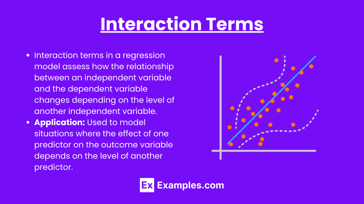
• Definition: Interaction terms in a regression model assess how the relationship between an independent variable and the dependent variable changes depending on the level of another independent variable.
• Application: Used to model situations where the effect of one predictor on the outcome variable depends on the level of another predictor.
• Example in Finance: Analyzing the interaction between economic growth and sector-specific factors on stock performance.

2. Polynomial Regression

• Definition: Polynomial regression extends linear regression by including higher-order terms (e.g., squared or cubic terms) of an independent variable to capture non-linear relationships.
• Application: Suitable when the relationship between the predictor and outcome variable is curved rather than linear.
• Example in Finance: Modeling the impact of age on asset depreciation, where the rate of depreciation decreases as the asset ages.

3. Dummy Variables

• Definition: Dummy variables are binary variables (taking values 0 or 1) that allow for the inclusion of categorical predictors in a regression model.
• Application: Enables the modeling of qualitative factors, such as industry classification or market conditions.
• Example in Finance: Using dummy variables to represent different industry sectors in a regression model for predicting stock returns.

4. Log-Linear and Log-Log Models

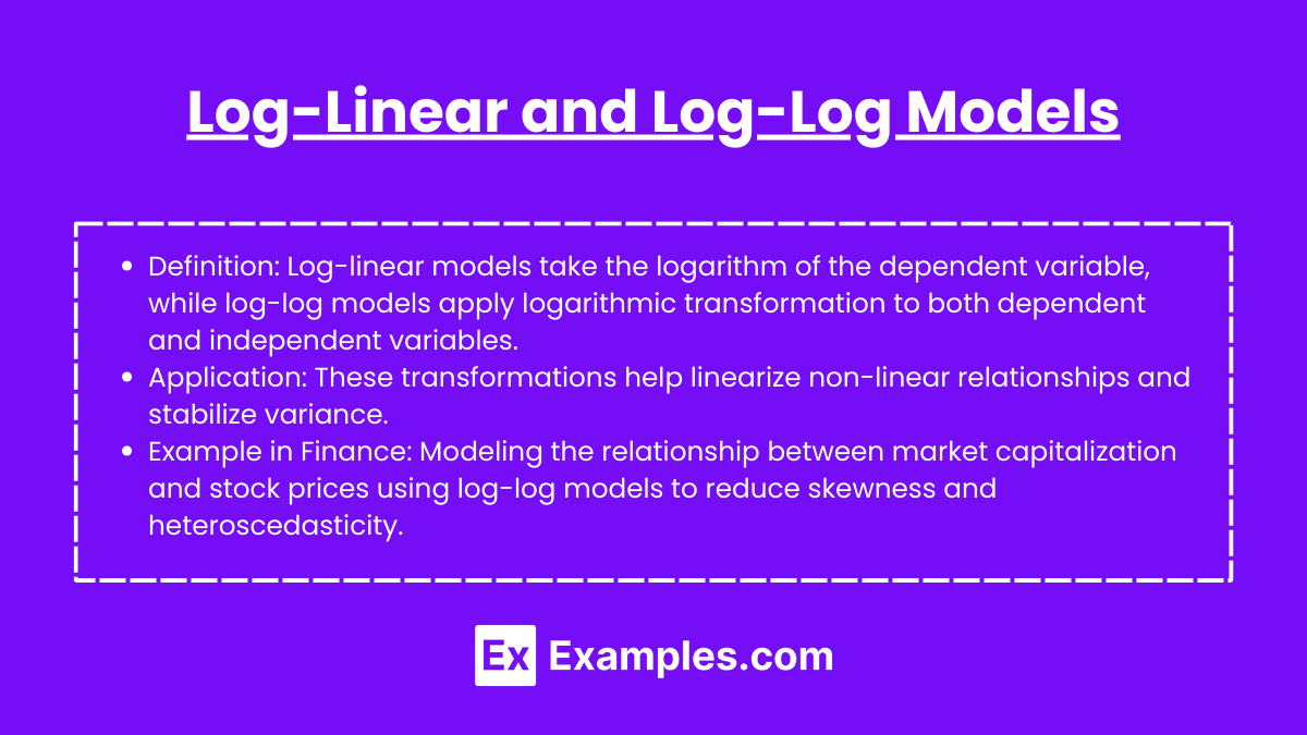
• Definition: Log-linear models take the logarithm of the dependent variable, while log-log models apply logarithmic transformation to both dependent and independent variables.
• Application: These transformations help linearize non-linear relationships and stabilize variance.
• Example in Finance: Modeling the relationship between market capitalization and stock prices using log-log models to reduce skewness and heteroscedasticity.

5. Addressing Multicollinearity with Ridge and Lasso Regression

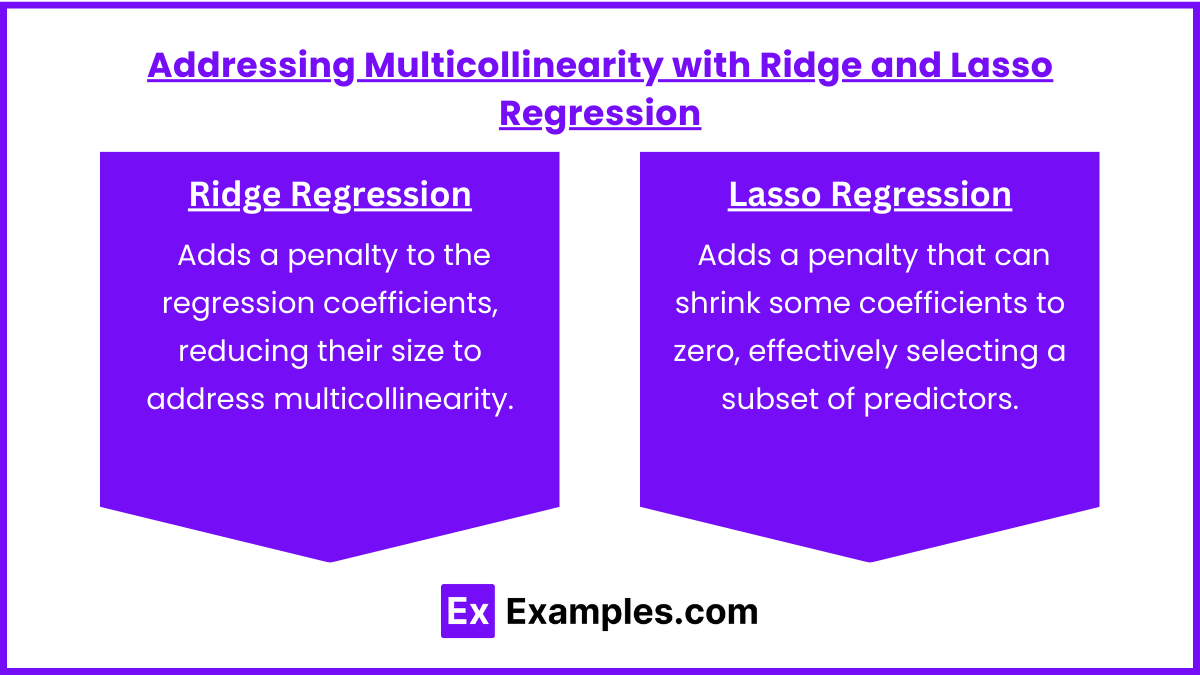
• Ridge Regression: Adds a penalty to the regression coefficients, reducing their size to address multicollinearity.
• Lasso Regression: Adds a penalty that can shrink some coefficients to zero, effectively selecting a subset of predictors.
• Example in Finance: Used when independent variables are highly correlated, such as in models incorporating overlapping economic indicators.

Examples

Example 1: Using Interaction Terms in Portfolio Analysis

• An analyst models portfolio returns based on sector and economic growth, including an interaction term to explore how growth influences different sectors uniquely.

Example 2: Applying Polynomial Regression for Asset Depreciation

• An economist uses polynomial regression to analyze the non-linear relationship between the age of machinery and its market value, capturing the decreasing rate of depreciation over time.

Example 3: Incorporating Dummy Variables in Stock Performance Analysis

• In a regression model predicting stock returns, an analyst uses dummy variables to account for industry sectors, isolating sector-specific effects on stock performance.

Example 4: Log-Log Model in Real Estate Pricing

• A real estate analyst applies a log-log model to predict property prices based on square footage, stabilizing the variance and reducing skewed data distribution.

Example 5: Ridge Regression in Predicting Economic Growth

• An economist uses ridge regression to manage multicollinearity among predictors in a model analyzing factors influencing GDP growth, balancing predictive power with model stability.

Practice Questions

Question 1

Which technique would best address a non-linear relationship between an independent and dependent variable?
A) Interaction terms
B) Dummy variables
C) Polynomial regression
D) Ridge regression

Answer: C) Polynomial regression

Explanation: Polynomial regression is specifically designed to model non-linear relationships by including higher-order terms, which allows for a better fit in cases where the relationship is not strictly linear.

Question 2:

What is the primary purpose of using dummy variables in a regression model?
A) To represent categorical variables
B) To address multicollinearity
C) To correct for heteroscedasticity
D) To transform the dependent variable

Answer: A) To represent categorical variables

Explanation: Dummy variables allow the inclusion of categorical data (e.g., industry sector or geographic location) in regression models, enabling analysts to account for qualitative factors without using numerical codes that might distort results.

Question 3:

Which regression technique helps address multicollinearity by penalizing the size of coefficients?
A) Log-linear models
B) Ridge regression
C) Dummy variables
D) Polynomial regression

Answer: B) Ridge regression

Explanation: Ridge regression applies a penalty to the size of the regression coefficients, which can reduce multicollinearity among predictors by shrinking their values, improving model stability.