“Portfolio Mathematics” in the CFA curriculum focuses on the quantitative analysis of investment portfolios, emphasizing risk and return measurement, diversification, and optimization techniques. This area explores fundamental concepts such as expected returns, portfolio variance, standard deviation, and covariance, which are essential for managing and evaluating portfolios. Additionally, candidates learn to apply models like the Capital Asset Pricing Model (CAPM) and performance metrics such as the Sharpe Ratio to optimize portfolios. Mastery of these tools enables professionals to make data-driven, strategic investment decisions that align with client objectives.

Free CFA Practice Test

Learning Objectives

In studying “Quantitative Methods: Portfolio Mathematics” for the CFA Exam, you should aim to understand the core principles of portfolio analysis, including calculating expected returns, portfolio variance, and standard deviation. Analyze how diversification, correlation, and covariance impact portfolio risk. Evaluate models such as the Capital Asset Pricing Model (CAPM) to assess risk and expected return, as well as optimization methods to construct efficient portfolios. Additionally, explore tools like Sharpe Ratio and beta, which assess portfolio performance relative to risk. Apply this knowledge to real-world portfolio scenarios, interpreting risk-return trade-offs, asset allocation, and performance metrics in CFA practice questions.

Portfolio mathematics is a critical component of quantitative methods in the CFA curriculum, essential for analyzing and managing investment portfolios effectively. The primary goal is to understand how to balance return and risk in a portfolio, optimize asset allocation, and measure portfolio performance. Key areas covered include the calculation of portfolio returns, portfolio risk, diversification benefits, the Capital Asset Pricing Model (CAPM), and the basics of portfolio optimization.

Portfolio Return Calculations

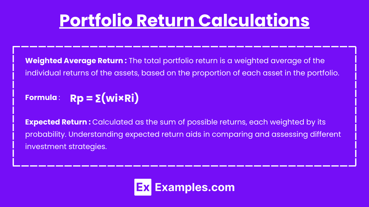
Weighted Average Return: The total portfolio return is a weighted average of the individual returns of the assets, based on the proportion of each asset in the portfolio.
- Formula: Rp=∑(wi×Ri)
- Where Rp is the portfolio return, wi is the weight of asset i, and Ri is the return of asset i.
Expected Return: Calculated as the sum of possible returns, each weighted by its probability. Understanding expected return aids in comparing and assessing different investment strategies.

Portfolio Risk and Variance

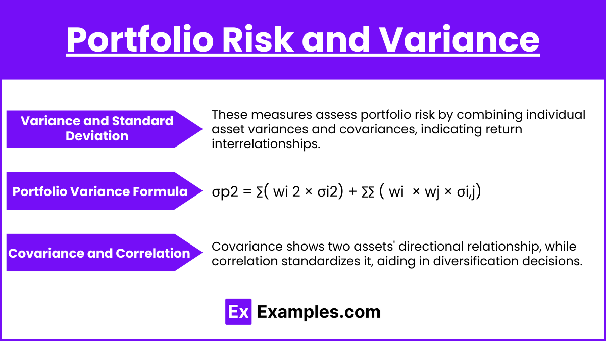
Variance and Standard Deviation: These measures assess the risk or volatility of a portfolio. They’re derived from the individual asset variances and covariances, which capture how asset returns move relative to each other.
- Portfolio Variance Formula: σ_p² = ∑( w_i ² × σ_i²) + ∑∑ ( w_i × w_j × σ_i,_j) Where σ_p² is the portfolio variance, w_i and w_j are weights of assets i and j, and σ_i,_j is the covariance between assets i and j.
Covariance and Correlation: Covariance measures the directional relationship between two assets, while correlation standardizes this relationship between -1 and 1, helping in diversification decisions.

Capital Allocation Line (CAL) and Optimal Portfolio Choice

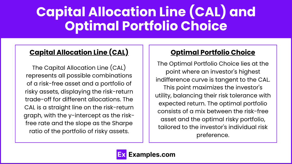
The Capital Allocation Line (CAL) represents all possible combinations of a risk-free asset and a portfolio of risky assets, displaying the risk-return trade-off for different allocations. The CAL is a straight line on the risk-return graph, with the y-intercept as the risk-free rate and the slope as the Sharpe ratio of the portfolio of risky assets. The slope indicates the additional return per unit of risk taken.
The Optimal Portfolio Choice lies at the point where an investor’s highest indifference curve is tangent to the CAL. This point maximizes the investor’s utility, balancing their risk tolerance with expected return. The optimal portfolio consists of a mix between the risk-free asset and the optimal risky portfolio, tailored to the investor’s individual risk preference. By choosing the optimal portfolio on the CAL, investors can achieve the best possible risk-adjusted return.

Practical Applications

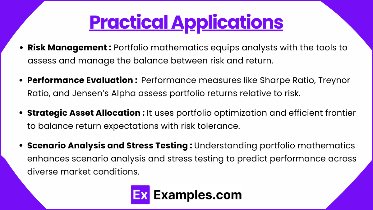
Risk Management
Portfolio mathematics equips analysts with the tools to assess and manage the balance between risk and return. Understanding correlations, betas, and asset weights enables effective diversification and risk control.
Performance Evaluation
Performance measures such as the Sharpe Ratio, Treynor Ratio, and Jensen’s Alpha are crucial for evaluating portfolio performance relative to its risk, providing insights into how well a portfolio meets its risk-return objectives.
Strategic Asset Allocation
Portfolio optimization and the efficient frontier concepts guide asset allocation decisions, helping investors achieve an optimal balance based on their return expectations and risk tolerance.
Scenario Analysis and Stress Testing
Understanding portfolio mathematics allows for better scenario analysis, helping to predict portfolio performance under various market conditions.

Examples

Example 1: Calculating Expected Portfolio Return

Imagine an investor holds a diversified portfolio consisting of equities, bonds, and commodities, each with different expected returns based on market predictions. By calculating the weighted average of these expected returns, the investor can estimate the portfolio’s overall expected return. For example, if equities have an expected return of 8%, bonds 4%, and commodities 6%, and the portfolio weights are 50%, 30%, and 20%, respectively, the expected portfolio return is calculated by combining these weighted returns, helping to project future growth potential for the portfolio.

Example 2: Assessing Portfolio Risk through Variance and Standard Deviation

An investor wants to understand the risk level of a portfolio composed of two assets with known individual risks and correlations. By applying portfolio variance and standard deviation formulas, the investor can calculate the total risk. For instance, if Asset A has a standard deviation of 12%, Asset B has 8%, and the correlation between them is 0.3, the investor can determine how these assets combine to reduce or increase total risk, supporting informed decision-making on asset allocation and risk management.

Example 3: Optimizing Asset Allocation on the Efficient Frontier

A portfolio manager aims to achieve an optimal balance of risk and return by allocating assets along the efficient frontier. By analyzing different asset combinations, they determine a mix of equities, bonds, and alternative investments that maximize return for a given level of risk. For example, an analysis might reveal that a 60% allocation in equities and 40% in bonds provides a higher expected return at acceptable risk, helping the manager to create a portfolio tailored to client risk tolerance and return expectations.

Example 4: Applying the Capital Asset Pricing Model (CAPM)

CAPM is used to assess whether an individual stock is fairly valued based on its risk relative to the market. For instance, an investor is considering adding Stock X to a portfolio. If the market’s expected return is 10%, the risk-free rate is 2%, and Stock X has a beta of 1.2, CAPM allows the investor to calculate Stock X’s expected return: 2% + 1.2 × (10% – 2%) = 11.6%. By comparing this expected return with Stock X’s current return, the investor can determine if Stock X offers sufficient compensation for its risk level, guiding investment decisions.

Example 5: Evaluating Portfolio Performance with the Sharpe Ratio

An investor wants to evaluate the risk-adjusted performance of two competing portfolios. By calculating each portfolio’s Sharpe Ratio, the investor can compare them based on their return per unit of risk. For example, if Portfolio A has an expected return of 9% and standard deviation of 10%, and Portfolio B has an expected return of 7% and standard deviation of 6%, with a risk-free rate of 2%, the Sharpe Ratios for Portfolio A and B would be calculated as (9% – 2%) / 10% = 0.7 and (7% – 2%) / 6% = 0.83, respectively. This analysis shows that Portfolio B offers a better risk-adjusted return, supporting decisions on which portfolio might better align with investment goals.

Practice Questions

Question 1

An investor has a portfolio with two assets, Asset A and Asset B. Asset A has an expected return of 10% with a weight of 60%, while Asset B has an expected return of 5% with a weight of 40%. What is the expected return of the portfolio?

A. 6%
B. 7%
C. 8%
D. 9%

Answer: C. 8%

Explanation:
The expected return of a portfolio is calculated as the weighted average of the returns of its individual assets. The formula is: $E(R_p) = w_A \cdot E(R_A) + w_B \cdot E(R_B)$

where:

w_A = 0.6 and E(R_A) = 10%
w_B = 0.4 and E(R_B) = 5%

Applying the values: E(Rp) = (0.6 × 10%) + (0.4 × 5%) = 6% + 2% = 8%

Therefore, the correct answer is C. 8%.

Question 2

A portfolio consists of two assets, X and Y, with standard deviations of 12% and 8%, respectively. If the weight of Asset X in the portfolio is 70%, the weight of Asset Y is 30%, and the correlation between X and Y is 0.25, what is the portfolio’s standard deviation?

A. 8.67%
B. 9.72%
C. 10.55%
D. 11.34%

Answer: B. 9.72%

Explanation:
The standard deviation of a two-asset portfolio is calculated using the formula:

$\sigma_p = \sqrt{(w_X \cdot \sigma_X)^2 + (w_Y \cdot \sigma_Y)^2 + 2 \cdot w_X \cdot w_Y \cdot \sigma_X \cdot \sigma_Y \cdot \rho_{X,Y}}$

where:

w_X=0.7, σ_X=12%
w_Y=0.3, σ_Y=8%
ρ_X,Y=0.25

Plugging in the values: Plugging in the values:
$\sigma_p = \sqrt{(0.7 \times 12\%)^2 + (0.3 \times 8\%)^2 + 2 \times 0.7 \times 0.3 \times 12\% \times 8\% \times 0.25}$

Calculating each term:

(0.7⋅12%)² = (8.4%)² = 0.07056
(0.3⋅8%)² = (2.4%)² = 0.00576
2⋅0.7⋅0.3⋅12%⋅8%⋅0.25 = 0.01008

Adding these values:σ_p = 0.07056 + 0.00576 + 0.01008 = 0.0864 = 9.72%

Thus, the correct answer is B. 9.72%.

Question 3

If an investor uses the Capital Asset Pricing Model (CAPM) to determine the expected return of a stock, which of the following factors is NOT directly used in the CAPM formula?

A. Beta of the stock
B. Risk-free rate
C. Expected market return
D. Standard deviation of the stock’s returns

Answer: D. Standard deviation of the stock’s returns

Explanation:
The Capital Asset Pricing Model (CAPM) formula is:

$E(R_i) = R_f + \beta_i \cdot (E(R_m) - R_f)$

where:

E(Ri) is the expected return of the stock
Rf is the risk-free rate
βi is the beta of the stock
E(Rm) is the expected market return

The standard deviation of the stock’s returns is not part of the CAPM formula. CAPM focuses on systematic risk, which is measured by beta, and does not account for total risk (systematic and unsystematic) as measured by standard deviation.

Therefore, the correct answer is D. Standard deviation of the stock’s returns.