Time-Series Analysis is a quantitative method used to analyze data points collected or recorded at specific time intervals, such as daily stock prices or monthly sales figures. By identifying patterns, trends, seasonality, and potential cycles within time series, analysts can make data-driven predictions and forecasts. Techniques like autoregressive (AR) and moving average (MA) models, along with combined models like ARIMA, help forecast future values by leveraging past data. Time-series analysis is essential for financial modeling, economic forecasting, and strategic planning, making it a critical skill for CFA candidates.

Free CFA Practice Test

Learning Objectives

In studying “Time-Series Analysis” for the CFA exam, you should learn to understand key methods for analyzing time-dependent financial data, including trends, seasonality, and autocorrelation. Explore models such as autoregressive (AR), moving average (MA), and autoregressive integrated moving average (ARIMA) to predict future values based on past data. Analyze how to use tools like the autocorrelation function (ACF) and partial autocorrelation function (PACF) to identify patterns and select the appropriate model. Additionally, evaluate the application of time-series analysis in forecasting financial variables, economic indicators, and asset prices, and apply these techniques to practical investment scenarios.

Time-series analysis allows analysts to examine past data to identify trends, seasonal patterns, and other time-dependent structures, enabling more accurate forecasting and decision-making. Key components of time-series analysis include trend, seasonality, stationarity, and autocorrelation, with common models like AR, MA, ARMA, and ARIMA used to model different types of data behavior.

1. Key Concepts in Time-Series AnalysisTrend

A trend represents a long-term increase or decrease in data over time. Trends may be linear (a steady increase or decrease) or nonlinear (growth or decay following a curve).
Identifying a trend is essential for determining the baseline direction of a time series and separating it from seasonal or cyclical components.

Seasonality

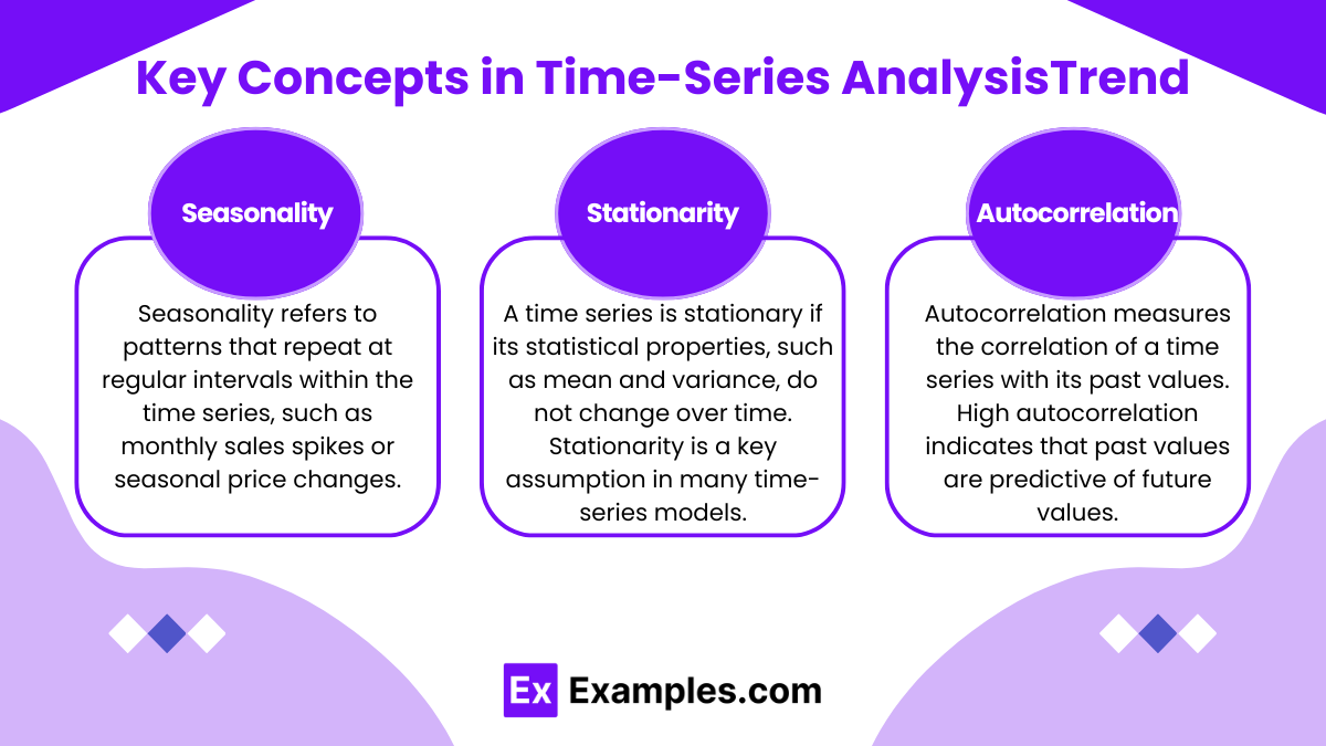
Seasonality refers to patterns that repeat at regular intervals within the time series, such as monthly sales spikes or seasonal price changes.
Seasonal adjustments are crucial for making data comparable across different periods and for accurate forecasting.

Stationarity

A time series is stationary if its statistical properties, such as mean and variance, do not change over time. Stationarity is a key assumption in many time-series models.
Differencing (subtracting the current value from the previous value) and log transformations are common techniques to make a time series stationary.

Autocorrelation

Autocorrelation measures the correlation of a time series with its past values. High autocorrelation indicates that past values are predictive of future values.
The autocorrelation function (ACF) and partial autocorrelation function (PACF) are tools for identifying the appropriate model for a time series by analyzing correlations at different lags.

2. Common Time-Series Models

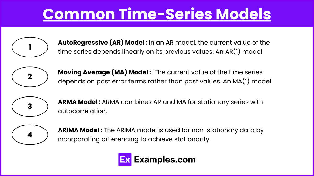
Several models are used in time-series analysis, depending on the nature of the data and the desired outcome. The most common models include AR (AutoRegressive), MA (Moving Average), ARMA (AutoRegressive Moving Average), and ARIMA (AutoRegressive Integrated Moving Average).

AutoRegressive (AR) Model

In an AR model, the current value of the time series depends linearly on its previous values. An AR(1) model, for example, would be: X_t = c + ϕX_t−1 + ϵ_twhere X_t is the current value, c is a constant, ϕ is the coefficient, and ϵ_t is a random error term.
The order of the AR model (AR(1), AR(2), etc.) indicates how many past observations are considered.

Moving Average (MA) Model

In an MA model, the current value of the time series depends on past error terms rather than past values. An MA(1) model, for example, would be: X_t = μ + θϵ_t−1 + ϵ_t where μ is the mean, θ is the coefficient, and ϵt and ϵ_t−1 are error terms.
The order of the MA model (MA(1), MA(2), etc.) indicates how many past error terms are included.

ARMA Model

The ARMA model combines both AR and MA components and is suitable for stationary series with autocorrelation and moving average components. An ARMA(1,1) model incorporates one lag of past values and one lag of error terms, making it flexible for various stationary series.

ARIMA Model

The ARIMA model is used for non-stationary data by incorporating differencing to achieve stationarity. ARIMA models are specified as ARIMA(p,d,q), where:
- p is the order of the autoregressive part,
- d is the degree of differencing needed to make the series stationary, and
- q is the order of the moving average part.
ARIMA is particularly useful for forecasting non-stationary series where trends need to be accounted for by differencing.

3. Seasonality and Exponential Smoothing

In addition to ARIMA, seasonal patterns in time-series data can be modeled with seasonal ARIMA (SARIMA) or exponential smoothing methods.

Seasonal ARIMA (SARIMA)

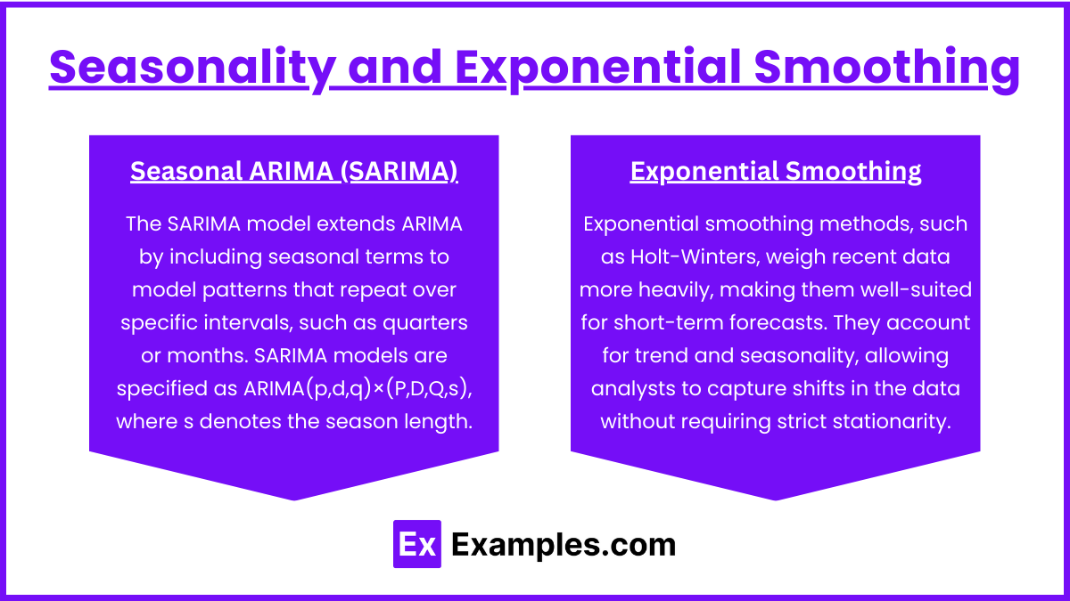
The SARIMA model extends ARIMA by including seasonal terms to model patterns that repeat over specific intervals, such as quarters or months. SARIMA models are specified as ARIMA(p,d,q)×(P,D,Q,s), where s denotes the season length.
Exponential smoothing methods, such as Holt-Winters, weigh recent data more heavily, making them well-suited for short-term forecasts. They account for trend and seasonality, allowing analysts to capture shifts in the data without requiring strict stationarity.

Exponential Smoothing

Exponential smoothing methods, such as Holt-Winters, weigh recent data more heavily, making them well-suited for short-term forecasts. They account for trend and seasonality, allowing analysts to capture shifts in the data without requiring strict stationarity.

4. Model Selection and Diagnostic Tools

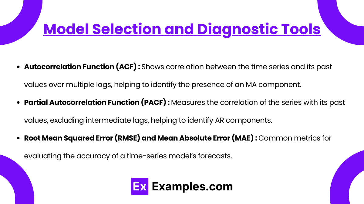
Selecting the right time-series model depends on the behavior of the data and the underlying patterns. Several diagnostic tools are used to identify the model’s fit:

Autocorrelation Function (ACF): Shows correlation between the time series and its past values over multiple lags, helping to identify the presence of an MA component.
Partial Autocorrelation Function (PACF): Measures the correlation of the series with its past values, excluding intermediate lags, helping to identify AR components.
Root Mean Squared Error (RMSE) and Mean Absolute Error (MAE): Common metrics for evaluating the accuracy of a time-series model’s forecasts.

Examples

Example 1: Trend Analysis in Economic Growth

An analyst examines annual GDP growth rates over the past 20 years, observing a steady upward trend despite short-term fluctuations. By fitting a linear regression model to the data, they project future GDP growth, accounting for both cyclical downturns and long-term growth. Recognizing trends in economic indicators allows analysts to make informed forecasts about a country’s economic outlook, an essential component of macroeconomic analysis.

Example 2: Seasonal Patterns in Tourism Revenue

A hospitality company tracks monthly revenue data over several years and notices consistent peaks during summer and winter holiday seasons. By applying a seasonal adjustment technique, such as decomposition, the analyst separates the trend, seasonal, and irregular components of the data. This approach helps the company accurately forecast revenue, allocate resources, and plan for high-demand periods. Seasonality is crucial for industries affected by predictable cyclical patterns.

Example 3: Modeling Inflation with AR(2) Process

To forecast monthly inflation rates, an economist uses an AR(2) model, where each month’s rate depends on the rates from the previous two months plus a random error. For example, the model might look like:

Inflation_t = 0.6⋅Inflation_t−1 + 0.3⋅Inflation_t−2 + ϵ_t

where ϵ_t represents the error term. This model accounts for persistence in inflation, where recent values influence future rates, helping the economist better predict inflation trends.

Example 4: Forecasting Stock Returns with ARIMA

A financial analyst analyzes daily returns of a stock index over the past five years. Due to apparent volatility and irregular trends, they apply an ARIMA(1,1,1) model, incorporating one differencing to achieve stationarity and one autoregressive and moving average term each. This model captures both trends and short-term dependencies, providing an effective framework for forecasting stock returns under changing market conditions, which is key for asset allocation and portfolio management.

Example 5: Using Exponential Smoothing for Sales Forecasting

A retailer observes monthly sales data, which shows recent increases in demand but has unpredictable short-term variations. They use exponential smoothing to weigh recent observations more heavily, allowing the model to quickly adapt to demand changes. This approach is particularly effective for short-term forecasts in fast-moving industries, enabling the retailer to adjust inventory levels and respond to demand shifts efficiently.

Practice Questions

Question 1

An analyst is examining quarterly sales data for a retail company over the last five years. The data shows consistent peaks in Q4 each year due to holiday shopping. Which time-series feature is most likely present in this data?

A. Trend
B. Seasonality
C. Random Walk
D. Mean Reversion

Answer: B. Seasonality

Explanation: Seasonality refers to recurring patterns in a time series that happen at regular intervals, such as quarterly or annually. In this case, the peaks in sales data during Q4 each year indicate a seasonal pattern due to holiday shopping. This predictable pattern repeats yearly, making seasonality the correct answer. Trend would indicate a long-term increase or decrease, random walk suggests a lack of pattern, and mean reversion implies a tendency to return to a long-term average, none of which best describe the consistent Q4 peaks observed here.

Question 2

An economist models monthly inflation rates using an AR(1) process. The model equation is given by:

Inflation_t = 0.7 × Inflation_t−1 + ϵ_t

where ϵ_t is a random error term. Which of the following statements is correct regarding this model?

A. The model is non-stationary due to the AR coefficient.
B. The model implies a mean-reverting process.
C. The model suggests that the inflation rate is unrelated to previous months.
D. The model will only produce accurate forecasts if the coefficient is greater than 1.

Answer: B. The model implies a mean-reverting process.

Explanation: In an AR(1) model, a coefficient less than 1 (in this case, 0.7) implies that the series will tend to revert toward its mean over time. This behavior is known as mean reversion, as the influence of past values diminishes, and the series tends to stabilize around a long-term average. The model is stationary because the coefficient is less than 1, ruling out A. The inflation rate in this model does depend on the previous month, making C incorrect. A coefficient greater than 1 would indicate non-stationarity, not improved accuracy, so D is incorrect.

Question 3

A financial analyst applies an ARIMA(1,1,1) model to forecast a non-stationary time series of stock returns. What does the “1,1,1” specification indicate about this model?

A. The model includes one autoregressive term, one differencing step, and one moving average term.
B. The model includes one moving average term and one seasonal adjustment.
C. The model requires one period of differencing to achieve seasonality.
D. The model has no autoregressive terms and relies solely on moving averages.

Answer: A. The model includes one autoregressive term, one differencing step, and one moving average term.

Explanation: An ARIMA(1,1,1) model specification denotes that the model includes one autoregressive term (AR), one differencing step (I), and one moving average term (MA). The differencing step is used to make the series stationary, which is necessary for non-stationary data like stock returns. This model captures both the autoregressive and moving average components of the time series, making A the correct answer. B and C are incorrect because they misinterpret the differencing component as a seasonal adjustment, while D incorrectly states that there are no autoregressive terms.