Understanding the “Valuation of Contingent Claims” is crucial for CFA Level 2 candidates, particularly for mastering derivatives. This topic involves the pricing of options and other contingent claims, employing models such as binomial and Black-Scholes. Proficiency in these models provides insight into hedging strategies and risk assessment in derivatives trading.

Free CFA Practice Test

Learning Objectives

In studying “Valuation of Contingent Claims” for the CFA, you will master foundational models and methodologies for pricing options and other contingent claims. You will analyze the binomial option pricing model, construct and calculate option trees, and apply the Black-Scholes-Merton model to European-style options while understanding factors like volatility, time to expiration, and interest rates. You will evaluate the Greeks to measure risk exposure and assess sensitivity to underlying variables, ultimately interpreting model results to make informed decisions in investment analysis and portfolio management.

1. Introduction to Contingent Claims

Contingent claims are financial instruments whose payoffs depend on the occurrence of a particular event in the future. These include options, warrants, and convertible securities, which are widely used in financial markets for hedging, speculation, and investment strategies. A contingent claim’s value changes with market conditions, particularly the price and volatility of the underlying asset. For CFA Level 2 candidates, understanding contingent claims is essential for evaluating and managing derivative-based strategies effectively. This knowledge equips them to assess and mitigate risks while capitalizing on opportunities offered by derivatives, enhancing their skill in structured finance and portfolio management.

2. Option Pricing Fundamentals

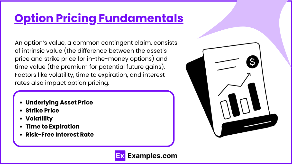
The value of an option, one of the most common types of contingent claims, is determined by two main components: intrinsic value and time value. Intrinsic value is the difference between the current price of the underlying asset and the option’s strike price (for in-the-money options) and represents the immediate payoff if the option were exercised. Time value, on the other hand, reflects the additional premium buyers are willing to pay for the possibility of the option increasing in value before expiration. Several factors impact option pricing, including:

Underlying Asset Price: Affects the intrinsic value as it fluctuates in the market.
Strike Price: Determines the threshold for option exercise.
Volatility: Higher volatility increases the option’s potential for profitability.
Time to Expiration: The more time an option has, the higher its time value.
Risk-Free Interest Rate: Impacts the present value of the strike price. Mastering these fundamentals provides a solid foundation for understanding and applying advanced option pricing models, helping candidates accurately assess and manage option positions.

3. Binomial Option Pricing Model

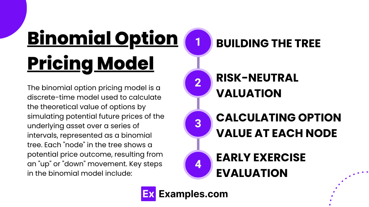
The binomial option pricing model is a discrete-time model used to calculate the theoretical value of options by simulating potential future prices of the underlying asset over a series of intervals, represented as a binomial tree. Each “node” in the tree shows a potential price outcome, resulting from an “up” or “down” movement. Key steps in the binomial model include:

Building the Tree: A binomial tree is constructed, with each node representing a potential price of the underlying asset.
Risk-Neutral Valuation: Probabilities are adjusted so that the expected price reflects the asset’s return as if it were risk-free.
Calculating Option Value at Each Node: By working backward from the final nodes to the root, option values are calculated using the risk-neutral probabilities and payoff formula.
Early Exercise Evaluation: This is especially relevant for American options, as the binomial model allows for the consideration of early exercise at each node. The binomial model’s step-by-step approach makes it particularly adaptable for various option types, including American-style options. However, the model becomes more complex with an increasing number of time intervals, which can limit its practicality for very high-frequency evaluations.

4. Black-Scholes-Merton Model

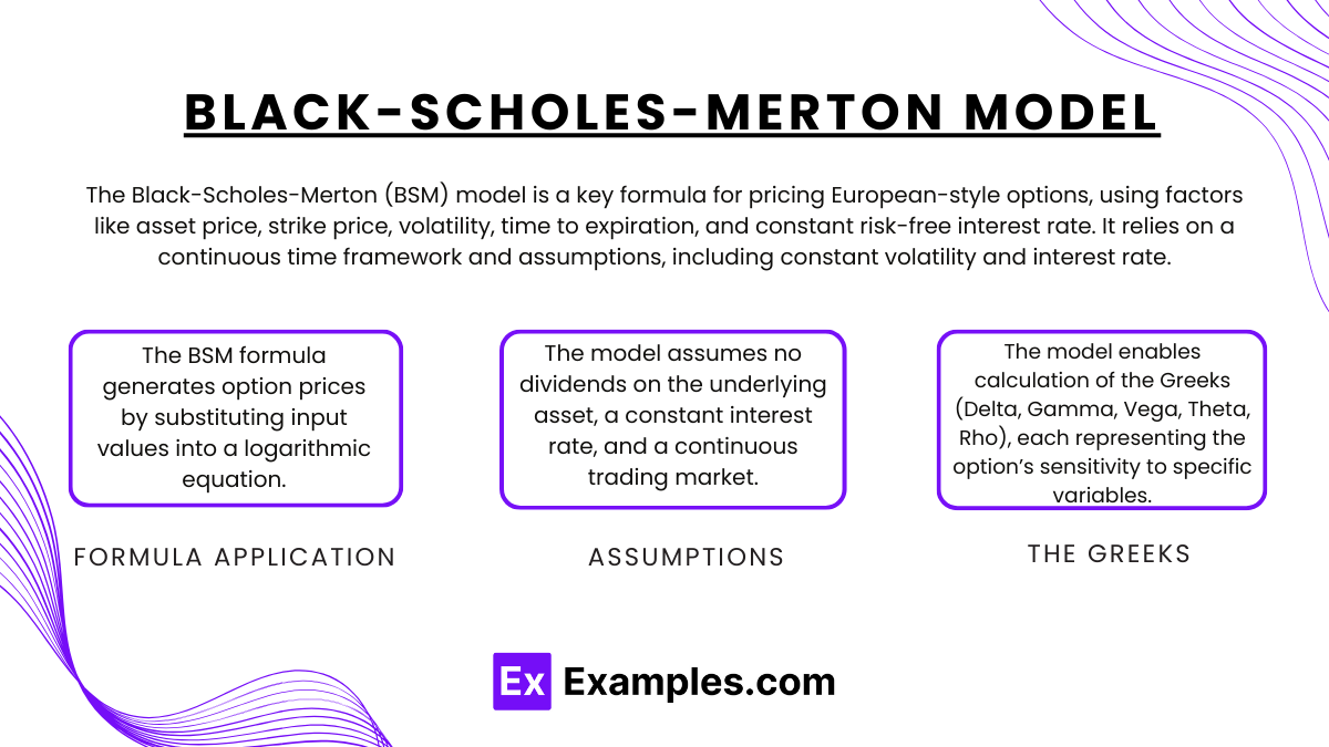
The Black-Scholes-Merton (BSM) model is a widely-used formula for pricing European-style options, relying on a continuous time framework and a set of assumptions, including constant volatility and a known, constant risk-free interest rate. The formula calculates the option price based on variables such as the underlying asset’s current price, strike price, volatility, time to expiration, and risk-free interest rate. Key components of the Black-Scholes model include:

Formula Application: The BSM formula generates option prices by substituting input values into a logarithmic equation.
Assumptions: The model assumes no dividends on the underlying asset, a constant interest rate, and a continuous trading market.
The Greeks: The model enables calculation of the Greeks (Delta, Gamma, Vega, Theta, Rho), each representing the option’s sensitivity to specific variables. Although the Black-Scholes model is efficient for European-style options, it has limitations, particularly in valuing American options due to its assumption of no early exercise. The model’s simplified assumptions also make it less accurate in highly volatile or unpredictable markets, though it remains one of the most popular methods due to its speed and effectiveness in stable conditions.

5. Risk Sensitivity and the Greeks

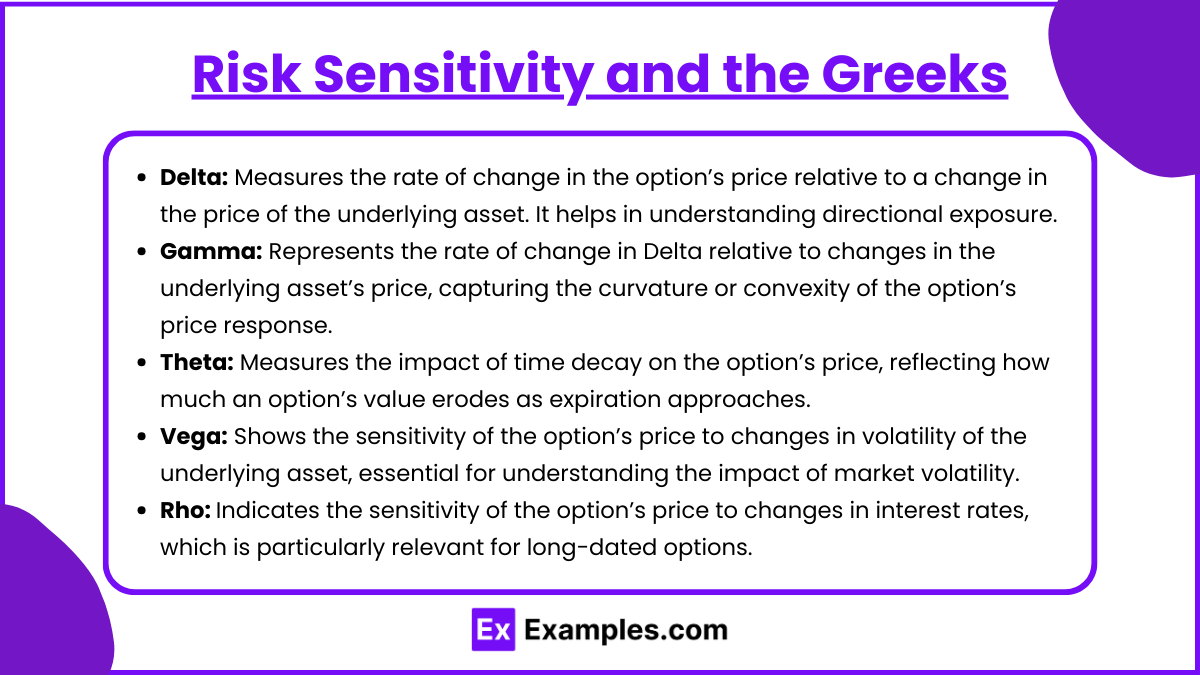
The Greeks are crucial metrics in option pricing that measure how various factors impact an option’s price, providing insights into the risk and sensitivity of a contingent claim’s value:

Delta: Measures the rate of change in the option’s price relative to a change in the price of the underlying asset. It helps in understanding directional exposure.
Gamma: Represents the rate of change in Delta relative to changes in the underlying asset’s price, capturing the curvature or convexity of the option’s price response.
Theta: Measures the impact of time decay on the option’s price, reflecting how much an option’s value erodes as expiration approaches.
Vega: Shows the sensitivity of the option’s price to changes in volatility of the underlying asset, essential for understanding the impact of market volatility.
Rho: Indicates the sensitivity of the option’s price to changes in interest rates, which is particularly relevant for long-dated options. Using the Greeks, investors can fine-tune their portfolios and hedge against specific risks by analyzing how each factor may influence the option’s price.

6. Practical Applications in Valuation

Valuing contingent claims has wide applications in risk management and strategic portfolio decisions. Financial professionals use valuation models to determine the fair value of options and to uncover potential arbitrage opportunities. For instance, options can be combined with underlying assets to construct hedging strategies, such as covered calls or protective puts, to safeguard against adverse price movements. Portfolio managers also use options for more sophisticated strategies like spreads and straddles, allowing for targeted risk and reward profiles. By mastering contingent claim valuation, CFA candidates are prepared to make informed investment decisions and improve the robustness of their portfolios.

Examples

Example 1

A trader wants to value a European call option on a stock. Given the stock price, strike price, risk-free rate, time to expiration, and volatility, apply the Black-Scholes-Merton model to find the option’s value.

Example 2

Using the binomial model, determine the value of a put option with a two-period tree. Explain the steps and calculations at each node.

Example 3

Analyze how an increase in volatility affects the price of a call option using the Black-Scholes model. Discuss the impact of the Vega on the option’s value.

Example 4

Calculate the Delta of an option and explain its role in hedging strategies. Show how Delta changes with variations in the stock price.

Example 5

Compare the valuation of an American option using the binomial model with the valuation of a European option using Black-Scholes. Discuss any discrepancies in values.

Practice Questions

Question 1

Which of the following models is primarily used for valuing European-style options?
A) Binomial Model
B) Monte Carlo Simulation
C) Black-Scholes Model
D) Real Options Valuation

Answer: C) Black-Scholes Model
Explanation: The Black-Scholes Model is commonly used for pricing European-style options due to its reliance on a continuous time framework, making it ideal for such applications.

Question 2

What does the “Gamma” of an option represent in derivatives valuation?
A) The sensitivity of the option’s price to changes in the volatility
B) The rate of change in the option Delta with respect to the underlying asset’s price
C) The option’s intrinsic value at expiration
D) The time decay of the option’s price

Answer: B) The rate of change in the option Delta with respect to the underlying asset’s price
Explanation: Gamma represents the sensitivity of Delta to changes in the underlying asset price, reflecting the non-linear relationship in option pricing.

Question 3

In the binomial option pricing model, the value of an option is determined by:
A) Adjusting the option’s strike price according to market conditions
B) Creating a replicating portfolio of the option using underlying assets and borrowing
C) Using only the historical volatility of the underlying asset
D) Taking the average price of the underlying asset over time

Answer: B) Creating a replicating portfolio of the option using underlying assets and borrowing
Explanation: The binomial model values an option by constructing a portfolio that replicates the option’s payoff, balancing the underlying asset and a risk-free borrowing position.