Preparing for the CFA Exam requires a thorough understanding of the “One-Period Binomial Model” for valuing derivatives, a fundamental approach in financial modeling. This model illustrates how a derivative’s value can be determined by considering possible price changes of the underlying asset over a single period. By assigning probabilities to upward and downward movements, the binomial model provides an intuitive framework for calculating potential derivative payoffs. Mastery of this model enables candidates to evaluate risk, hedge effectively, and make informed decisions about options and other derivatives. This foundational knowledge is crucial for achieving a high CFA score.

Free CFA Practice Test

Learning Objectives

In studying “Valuing a Derivative Using a One-Period Binomial Model” for the CFA, you should aim to grasp the foundational concepts of modeling price movements to assess derivative value. This approach involves estimating potential price shifts of the underlying asset over a single time period, which provides a structured method for calculating the derivative’s expected payoff. By understanding how to assign probabilities to upward and downward movements, you can determine the option’s fair value and manage risk more effectively. Mastery of this model allows you to evaluate derivatives with greater precision and make more informed financial decisions.

Understanding the Binomial Model Framework

The binomial model is designed to forecast potential future prices of an asset over discrete time intervals, such as a single period. In this one-period model, the asset’s price can take one of two possible paths: an upward movement or a downward movement, commonly represented as “up” and “down” states. This dichotomy mirrors the random nature of market price movements, allowing investors to assess a range of possible outcomes. These price movements are typically based on two essential factors:

The Upward Price Movement (U): Represents the factor by which the price increases.
The Downward Price Movement (D): Represents the factor by which the price decreases.

Each of these price outcomes is accompanied by a probability estimate, which reflects the likelihood of the price moving up or down in the given period.

Applications of Valuing a Derivative Using a One-Period Binomial Model

Valuing a derivative using a one-period binomial model has several practical applications, particularly in finance. Here are some key applications:

Option Pricing
- The binomial model is commonly used to value stock options, including call and put options. In this application, the model estimates the potential future prices of the underlying asset (e.g., stock) over a single time period, enabling analysts to compute the value of the option at each node and ultimately determine its fair value.
Risk Management
- Derivative valuation using the binomial model can support risk management strategies. By understanding the potential values of derivatives, financial professionals can hedge against unfavorable price movements in underlying assets. For instance, they might calculate the appropriate number of options or futures contracts needed to hedge a position.
Portfolio Management and Asset Allocation
- Portfolio managers use the binomial model to estimate future price ranges of assets, helping them decide on asset allocations. For example, they may use derivatives priced with this model to balance risk and return in an equity-heavy portfolio.
Pricing Convertible Securities
- The model can be applied to value convertible bonds, which are hybrid securities with debt and equity characteristics. The model helps estimate the value of the bond in different scenarios, including potential future conversion to equity, enabling better pricing and investment decisions.
Valuing Employee Stock Options (ESOs)
- Companies often use the binomial model to value employee stock options granted as part of compensation packages. This helps companies determine the cost associated with these options and manage their financial reporting more accurately under accounting standards like FASB and IFRS.

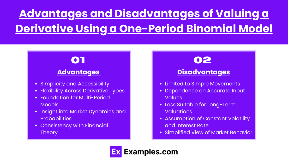
Advantages and Disadvantages of Valuing a Derivative Using a One-Period Binomial Model

Advantages of Valuing a Derivative Using a One-Period Binomial Model

Simplicity and Accessibility
The one-period binomial model is straightforward and intuitive, making it accessible for both novice and experienced investors. It requires minimal mathematical complexity, offering a clear and structured approach to option valuation.
Flexibility Across Derivative Types
While commonly used for options, the one-period model can be adapted for various other derivative instruments, making it versatile within financial modeling.
Foundation for Multi-Period Models
The one-period model serves as the basis for more advanced models, such as the multi-period Cox-Ross-Rubinstein binomial model. By understanding the single-period model, analysts can extend this logic to multi-step evaluations, allowing for the valuation of options over longer time frames.
Insight into Market Dynamics and Probabilities
The model incorporates risk-neutral probabilities, helping investors understand the balance of potential risks and rewards under market conditions. This offers a simplified yet insightful way to see how probability factors into pricing.
Consistency with Financial Theory
By incorporating risk-neutral probabilities, the binomial model aligns with fundamental financial principles. This consistency allows for a theoretically sound approach that aligns derivative pricing with market risk expectations and interest rates.

Disadvantages of Valuing a Derivative Using a One-Period Binomial Model

Limited to Simple Movements
The model assumes only two possible price paths (up and down) for the underlying asset, which is an oversimplification of real-world market dynamics where multiple outcomes are possible. This can lead to inaccurate estimates for derivatives sensitive to more nuanced price fluctuations.
Dependence on Accurate Input Values
The effectiveness of the model relies heavily on precise input values for the upward and downward price movements and the risk-free rate. Any inaccuracies in these inputs can significantly affect the model’s output, leading to unreliable valuations.
Less Suitable for Long-Term Valuations
Since it evaluates only a single period, the model may not be ideal for long-term options or derivatives, which typically require a multi-period framework to capture potential variations over time. A single-period model may miss the complexities of extended time horizons.
Assumption of Constant Volatility and Interest Rate
The model assumes that volatility and interest rates remain constant during the period, which may not reflect real market conditions. This limits its accuracy in dynamic markets where these factors can vary significantly.
Simplified View of Market Behavior
Real-world markets exhibit complexities that cannot be captured by a binary up-or-down approach. Events such as sharp market corrections, interest rate shifts, and economic announcements can affect prices in non-binary ways, which the one-period model cannot easily account for.

Calculating Expected Payoff and Valuation

The one-period binomial model requires the calculation of the option’s payoff at each possible end-of-period price. To calculate the expected payoff, we evaluate the potential gains (or losses) from the option if the price moves up or down. Once the payoffs for each scenario are computed, we calculate the expected value of the option by weighing each outcome by its respective probability.

To achieve an accurate expected value, the model uses a risk-neutral probability (also called the “risk-adjusted” probability), which assumes investors are indifferent to risk. The risk-neutral probability q is calculated using:
$q = \frac{(1 + r) - D}{U - D}$

where:

r is the risk-free rate over the period,
U is the factor for upward movement,
D is the factor for downward movement.

Determining the Option Price

The option price at the beginning of the period is determined by discounting the expected payoff by the risk-free rate. This process reflects the time value of money, ensuring that the valuation aligns with present values rather than future estimates. The formula for the option’s current value V₀is:
$V_0 = \frac{1}{1 + r} \left( q \cdot V_{\text{up}} + (1 - q) \cdot V_{\text{down}} \right)$

where:

V_up is the payoff if the price goes up,
V_downis the payoff if the price goes down.

By this formula, the model applies the weighted average of the possible future payoffs, adjusted to the present using the risk-free rate. This is a critical step in aligning derivative values with fundamental pricing principles.

Examples

Example 1. Hedging Strategies for Options

By using a one-period binomial model, financial analysts can calculate the value of options for hedging purposes. This involves creating a portfolio of the option and the underlying asset that perfectly replicates the option’s payoff, thus allowing investors to mitigate risks associated with price fluctuations. The model helps determine the appropriate proportion of assets needed to offset risks, which is invaluable for managing portfolios in volatile markets.

Example 2. Risk-Neutral Valuation in Derivatives Trading

The one-period binomial model is instrumental in implementing risk-neutral valuation techniques, where the probability of price movements is adjusted so that the expected return of the underlying asset is the risk-free rate. This simplifies the valuation process and is commonly used in pricing derivatives like call and put options, making it a fundamental approach in derivatives trading and financial modeling.

Example 3. Assessing Pricing in Volatile Markets

Financial institutions often use the one-period binomial model to evaluate derivative prices when dealing with assets in highly volatile markets. The model provides a simplified framework for anticipating potential price changes over a short period, allowing traders to set fair prices for derivatives and to understand the potential payoffs for different market scenarios, contributing to more informed trading decisions.

Example 4. Academic and Practical Training for Financial Analysts

In academic and corporate training environments, the one-period binomial model serves as an introductory approach to understanding complex derivatives pricing. By learning to apply this model, analysts gain foundational knowledge in financial mathematics, enabling them to expand to more sophisticated models like multi-period binomial trees and the Black-Scholes model, which are essential for advanced financial analysis.

Example 5. Real Options Analysis for Corporate Decision-Making

Companies employ the one-period binomial model in real options analysis to evaluate investment opportunities, treating them as options. This approach allows firms to value strategic decisions, such as delaying or expanding a project, under uncertain market conditions. By modeling potential future outcomes, the binomial model provides corporate managers with insights into the value of flexibility in investment decisions.

Practice Questions

Question 1

What is the first step in valuing a derivative using a one-period binomial model?

A) Determining the probabilities of the stock price going up or down
B) Calculating the risk-neutral probability
C) Setting up the possible stock price changes over the period
D) Calculating the derivative’s payoff at maturity

Answer: C) Setting up the possible stock price changes over the period

Explanation: The first step in using a one-period binomial model is to outline the potential future prices of the underlying asset, which is generally a stock. In a one-period model, the stock can either move up by a factor (often denoted by uuu) or down by a factor (denoted by ddd). This setup creates two possible end-of-period stock prices, which are essential for calculating the value of a derivative. Once the possible prices are established, the model can proceed to determine the payoff and calculate risk-neutral probabilities.

Question 2

In a one-period binomial model, which of the following is correct about the “risk-neutral probability”?

A) It is the actual probability of the stock price moving up.
B) It is a theoretical probability that ensures the expected return matches the risk-free rate.
C) It is only used to calculate the option payoff in the real-world context.
D) It represents the probability that maximizes the stock price at maturity.

Answer: B) It is a theoretical probability that ensures the expected return matches the risk-free rate.

Explanation: In a binomial model, the “risk-neutral probability” is not the actual probability of stock movement but a theoretical construct that allows for pricing derivatives in a way that aligns the expected return of the asset with the risk-free rate. This probability ensures that under a “risk-neutral” framework, the value of the derivative can be calculated independently of the real-world probabilities. The risk-neutral probability is determined based on the possible up and down movements of the stock and the risk-free rate, facilitating the valuation of the option or derivative without speculating on actual market behavior.

Question 3

In the context of a one-period binomial model, why is it important to use the risk-neutral probability rather than the actual probability of price movement?

A) To ensure that the model’s results match real-world outcomes.
B) To adjust for the risk preference of individual investors.
C) To value the derivative in a way that reflects only the time value of money and not individual risk preferences.
D) To incorporate market sentiment into the option price.

Answer: C) To value the derivative in a way that reflects only the time value of money and not individual risk preferences.

Explanation: The use of risk-neutral probability in the binomial model is essential because it simplifies the valuation process by neutralizing the effect of investors’ risk preferences. By adopting a risk-neutral approach, the model calculates the derivative’s price based solely on the time value of money, aligning the expected return of the underlying asset with the risk-free rate. This approach allows for a consistent and objective pricing framework without needing to predict actual market movements or investor behavior, thus providing a purely financial valuation of the derivative.