Descriptive statistics summarize and analyze data, allowing for a clear understanding of central tendencies, variability, and data distribution. In finance, descriptive statistics are essential for interpreting historical performance, assessing risk, and identifying patterns. Key measures include mean, median, mode, standard deviation, skewness, and kurtosis, each revealing insights into trends, volatility, and potential anomalies within data. By understanding these metrics, analysts gain a foundational grasp of data behavior, which aids in making informed decisions, particularly useful in fields like the CFA for risk assessment and market analysis.
Learning Objectives
In studying “Introduction to Descriptive Statistics” for the CMT Exam, you should learn to understand the core principles and methods used to summarize and interpret market data. Examine measures of central tendency, such as mean, median, and mode, and measures of dispersion, including range, variance, and standard deviation, to assess price volatility and trends. Evaluate the significance of skewness and kurtosis for identifying distribution shapes, as well as correlation and covariance to understand asset relationships. Additionally, explore how these statistical tools assist in identifying patterns, evaluating market conditions, and making informed trading decisions, applying these concepts to practical CMT exam scenarios.
Descriptive Statistics for Technical Analysts

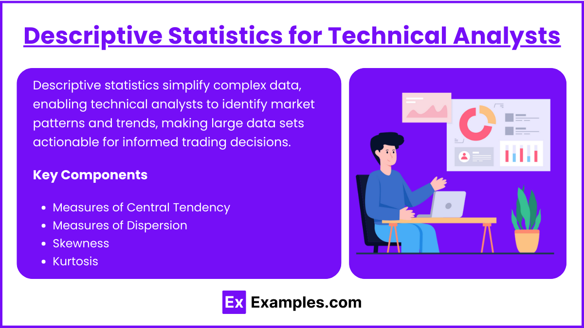
Descriptive statistics summarize and analyze historical data, helping technical analysts to identify underlying patterns and behavioral characteristics in markets. This branch of statistics organizes and simplifies large data sets, transforming them into meaningful information that guides trading decisions. By breaking down complex price movements and indicators into key metrics, descriptive statistics empower technical analysts to make sense of past data, gauge current trends, and anticipate potential price movements.
Key Components
- Measures of Central Tendency
- Measures of Dispersion
- Skewness
- Kurtosis
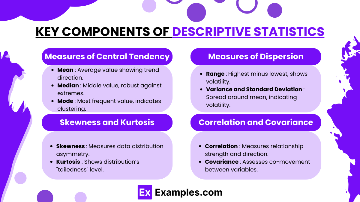
Key Components of Descriptive Statistics

- Measures of Central Tendency
- Mean: The average value of a data set, useful for identifying the overall direction of a trend in a market or security. For technical analysts, the mean helps identify typical price levels.
- Median: The middle value, which can be more reliable in skewed data sets as it is less affected by extreme values. Analysts use the median to locate the central tendency in non-normally distributed price data.
- Mode: The most frequent value, indicating the level where prices have often clustered, providing insights into common price levels.
- Measures of Dispersion
- Range: The difference between the highest and lowest values, offering a basic view of price volatility.
- Variance and Standard Deviation: These metrics show how spread out prices are around the mean. Standard deviation, in particular, is frequently used in technical analysis to gauge volatility and identify periods of high or low market risk.
- Skewness and Kurtosis
- Skewness measures the asymmetry of a data distribution. In technical analysis, skewness helps understand if returns have a long tail on one side, indicating the likelihood of extreme price movements.
- Kurtosis indicates the “tailedness” of a distribution. High kurtosis suggests a data set with more extreme values, often seen in market conditions with sudden price jumps or crashes.
- Correlation and Covariance
- Correlation measures the strength and direction of a relationship between two variables. For technical analysts, correlation between different securities or indices can indicate interconnectedness within markets.
- Covariance evaluates how two variables change together, helping analysts anticipate how one security may respond to changes in another, a crucial element in risk management and portfolio diversification.
Application of Descriptive Statistics in Technical Analysis

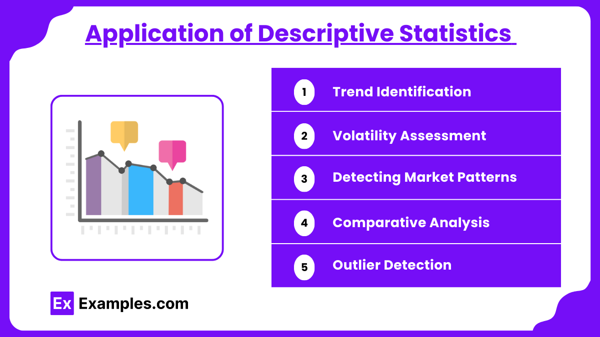
- Trend Identification
By calculating the mean price of a security over time, analysts can establish the underlying trend. Standard deviation assists in assessing whether price fluctuations are deviating from the trend, allowing technical analysts to make informed decisions on potential entry and exit points. - Volatility Assessment
Standard deviation and range provide insights into a security’s volatility, a key factor in assessing the risk associated with a particular asset. This knowledge is crucial for setting appropriate stop-loss and take-profit levels in a trade. - Detecting Market Patterns
Patterns such as head and shoulders or support and resistance levels often emerge from visualizations created through descriptive statistics. Analysts look for clustering around these levels to confirm or challenge the likelihood of an ongoing trend. - Comparative Analysis
Using covariance and correlation, technical analysts can study interrelationships between various assets. This is particularly useful in portfolio management, where analysts seek assets with low or negative correlation to diversify risk effectively. - Outlier Detection
Outliers in a data set may signify rare but impactful market events, such as sudden price surges or drops. Understanding skewness and kurtosis helps analysts recognize these outliers and assess their impact on the overall analysis.
Examples
Example 1: Mean Price Calculation
Technical analysts often calculate the mean price of a security over a given period (e.g., 20 days) to establish a baseline trend. If the mean is steadily increasing, it suggests an upward trend, while a decreasing mean indicates a downtrend. This can be used as a simple moving average to help set entry and exit points, with the mean serving as a central tendency around which prices fluctuate.
Example 2: Standard Deviation for Volatility
Standard deviation is crucial for measuring price volatility. In technical analysis, a higher standard deviation indicates more significant price swings, which may signal potential risk or opportunity depending on the analyst’s strategy. For example, Bollinger Bands apply standard deviations above and below a moving average to visualize price volatility and identify potential breakouts.
Example 3: Skewness in Price Returns
Analyzing skewness in a stock’s return distribution can indicate the likelihood of extreme price movements. Positive skewness implies more frequent small losses with occasional large gains, which might suit certain risk profiles. Conversely, a negative skew suggests the presence of more frequent gains with potential for sudden, large drops, warning of downside risk for traders.
Example 4: Correlation Between Securities
Technical analysts examine correlation to understand relationships between different assets. For instance, a high positive correlation between a tech stock and a tech-focused ETF could suggest that the stock will likely follow broader industry trends. Conversely, a low or negative correlation between two assets supports diversification, as one asset may act as a hedge against the other’s volatility.
Example 5: Range for Support and Resistance Levels
The range, or difference between the highest and lowest prices, helps identify potential support and resistance levels. For example, if a stock repeatedly fluctuates within a specific price range, analysts may consider the high and low ends of this range as resistance and support levels, respectively. These levels provide insights into likely price boundaries and points where the stock might reverse or break out, guiding trading decisions.
Practice Questions
Question 1
Which of the following measures of central tendency is most resistant to extreme outliers?
A) Mean
B) Median
C) Mode
D) Standard Deviation
Answer: B) Median
Explanation: The median is the middle value in a sorted data set and is not influenced by extreme outliers, making it more resistant to distortion from unusually high or low values compared to the mean. In technical analysis, using the median can provide a better representation of central price levels when a security’s price has high volatility or extreme price movements. The mean, on the other hand, is sensitive to outliers and can shift significantly due to extreme values, whereas the mode simply identifies the most frequent value, not necessarily the center. Standard deviation is not a measure of central tendency but rather a measure of dispersion.
Question 2
Which of the following best describes kurtosis in the context of price returns?
A) It measures the asymmetry of the distribution.
B) It indicates the degree of peakedness and tail heaviness in the distribution.
C) It calculates the average spread of data points from the mean.
D) It assesses the correlation between two assets.
Answer: B) It indicates the degree of peakedness and tail heaviness in the distribution.
Explanation: Kurtosis is a statistical measure that describes the distribution’s shape, specifically focusing on the “tails” and the “peak” relative to a normal distribution. In financial contexts, high kurtosis (leptokurtic distribution) suggests more data points in the tails, indicating a higher likelihood of extreme returns, which can mean increased market risk. Low kurtosis (platykurtic distribution) implies fewer outliers. Option A describes skewness, option C describes standard deviation (dispersion measure), and option D is unrelated to kurtosis, as it refers to correlation.
Question 3
A technical analyst is comparing the price movements of two stocks and calculates a correlation coefficient of -0.8. What does this value indicate about the relationship between the two stocks?
A) The stocks move in the same direction strongly.
B) The stocks have no relationship.
C) The stocks move in opposite directions strongly.
D) The stocks have low volatility.
Answer: C) The stocks move in opposite directions strongly.
Explanation: A correlation coefficient ranges from -1 to +1. A value of -0.8 indicates a strong negative correlation, meaning that as the price of one stock tends to increase, the price of the other stock tends to decrease. This negative relationship can be useful in diversification strategies, where selecting assets with negative correlations may reduce portfolio risk. Option A would be correct if the correlation were positive and close to +1, Option B would be correct if the correlation were close to 0, and Option D is unrelated, as correlation does not directly measure volatility.


