One-Variable Data: Distributions and Measures of Center and Spread

One-variable data, also known as univariate data, consists of observations on a single characteristic or attribute. In the context of the Digital SAT Exam, understanding one-variable data involves analyzing distributions and calculating measures of center and spread. These concepts are fundamental in statistics, enabling students to summarize and interpret data effectively. Distributions provide a visual representation of data, while measures of center (mean, median, mode) and spread (range, interquartile range, standard deviation) offer quantitative summaries that describe the data’s central tendency and variability.

Learning Objectives

In this section, you will learn how to describe and analyze distributions of one-variable data, calculate and interpret measures of center and spread, and apply these concepts to real-world scenarios. By the end of this section, you will be able to effectively summarize data sets and interpret statistical results, skills that are essential for the Digital SAT Exam and beyond.

One-Variable Data: Distributions

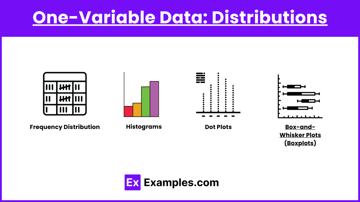
A distribution shows how the values of a variable are spread or distributed. It can be represented in various ways, including tables, graphs, and charts. The most common types of distributions for one-variable data include:

Frequency Distribution: A table that displays the frequency (or count) of observations within specific intervals.
Histogram: A graphical representation of a frequency distribution, where data is grouped into bins or intervals, and the height of each bar represents the frequency.
Dot Plot: A simple graph that shows individual data points plotted above a number line.
Box Plot (Box-and-Whisker Plot): A graphical summary that shows the distribution of data based on a five-number summary (minimum, Q1, median, Q3, maximum).

Example: Creating a Frequency Distribution

Consider the data set: 2, 3, 3, 4, 5, 5, 5, 6, 7, 7

Identify the range of the data: 2 to 7.
Create intervals (bins) for the data, such as 2-3, 4-5, 6-7.
Count the number of observations in each bin.
Display the frequencies in a table.

Interval	Frequency
2-3	3
4-5	4
6-7	3

One-Variable Data: Measures of Center

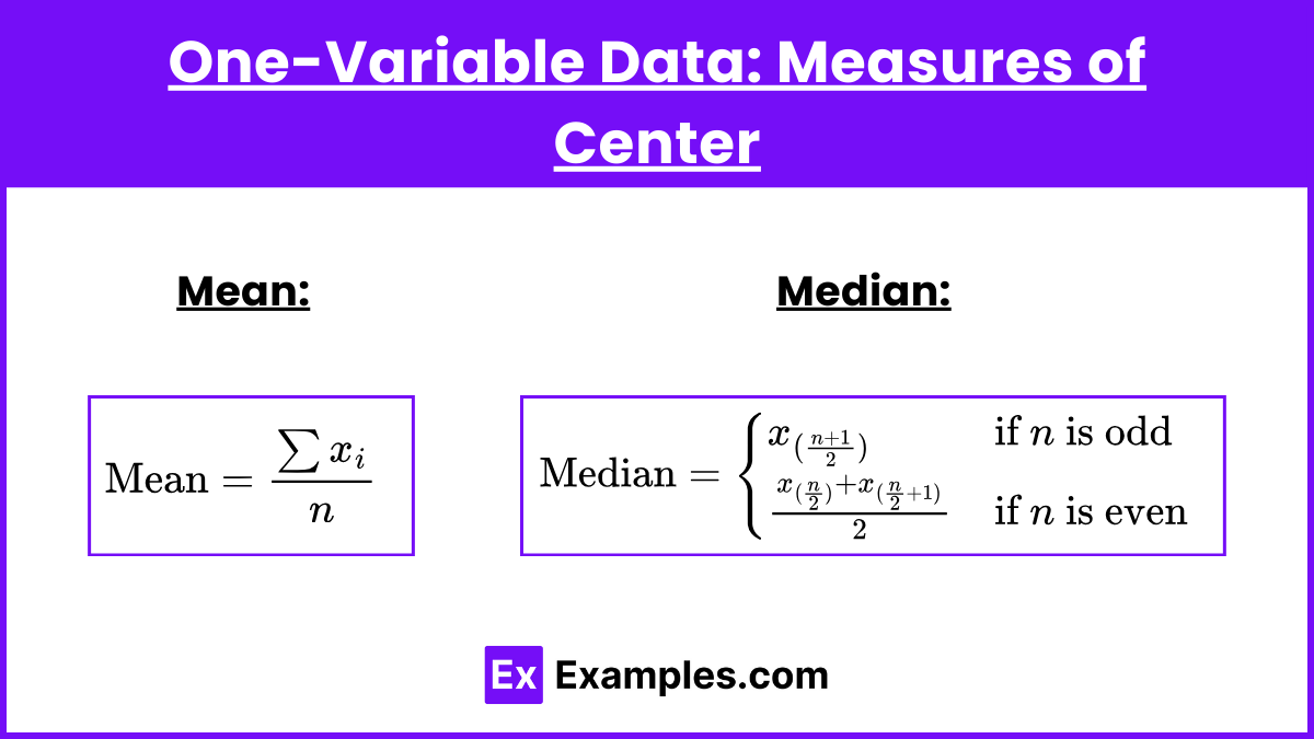
Measures of center, also known as measures of central tendency, describe the central point of a data set. The three main measures of center are:

Mean (Average): The sum of all data values divided by the number of values. It is sensitive to outliers.

\[ \text{Mean} = \frac{\sum x_i}{n} \]
where xᵢ represents each data value and nnn is the number of data values.

Median: The middle value when the data is ordered from least to greatest. If there is an even number of values, the median is the average of the two middle values. It is less sensitive to outliers.
\[ \text{Median} = \begin{cases} x_{(\frac{n+1}{2})} & \text{if } n \text{ is odd} \\ \frac{x_{(\frac{n}{2})} + x_{(\frac{n}{2}+1)}}{2} & \text{if } n \text{ is even} \end{cases} \]
Mode: The value(s) that occur most frequently in the data set. A data set may have no mode, one mode, or multiple modes.

One-Variable Data: Measures of Spread

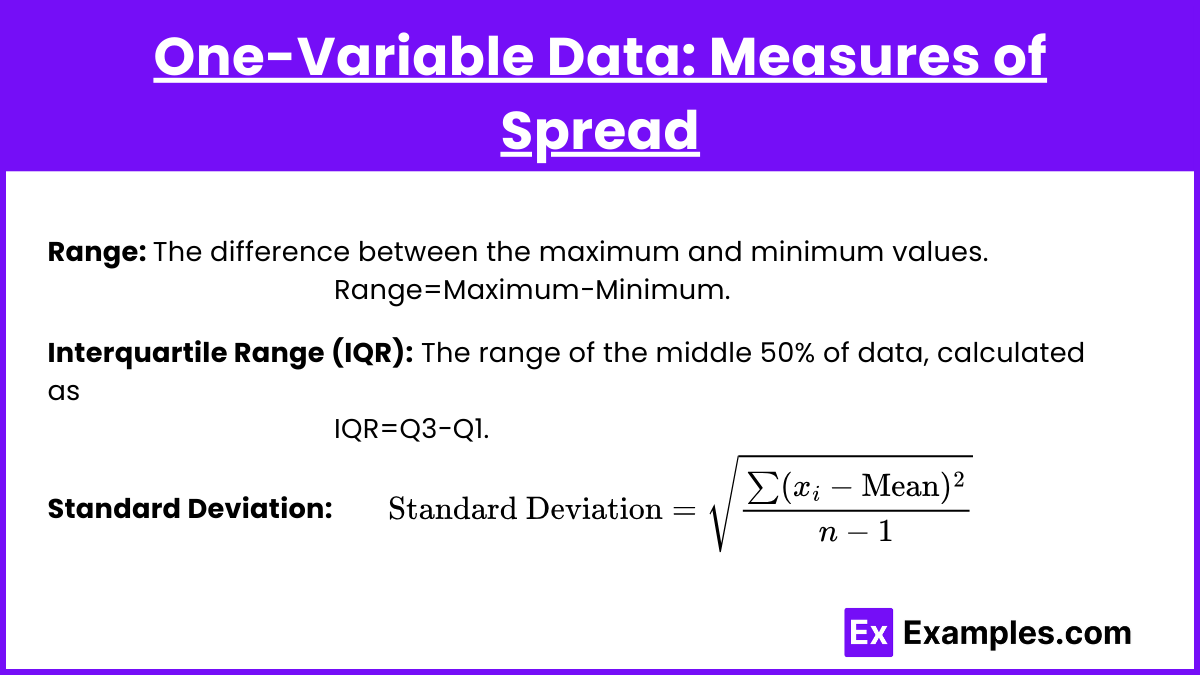
Measures of spread describe the variability or dispersion of a data set. The main measures of spread include:

Range: The difference between the maximum and minimum values.
Range=Maximum−Minimum
Interquartile Range (IQR): The range of the middle 50% of the data, calculated as the difference between the third quartile (Q3) and the first quartile (Q1).
IQR=Q3−Q1
Standard Deviation: A measure of the average distance of each data point from the mean. It is calculated as the square root of the variance.
\[ \text{Standard Deviation} = \sqrt{\frac{\sum (x_i – \text{Mean})^2}{n-1}} \]

where xᵢ represents each data value, and n is the number of data values.

Real-World Applications

Understanding distributions and measures of center and spread is essential in various fields such as economics, healthcare, engineering, and social sciences. For example, in healthcare, analyzing the distribution of patient ages and calculating measures of center and spread can help identify trends and allocate resources effectively.

Examples

Example 1: Calculating Mean, Median, and Mode

Consider the data set: 3, 7, 7, 2, 9

Mean: \[ \text{Mean} = \frac{3 + 7 + 7 + 2 + 9}{5} = \frac{28}{5} = 5.6 \]
Median: Order the data: 2, 3, 7, 7, 9. The middle value is 7, so the median is 7.
Mode: The value 7 appears most frequently, so the mode is 7.

Example 2: Calculating Range and IQR

Consider the data set: 4, 8, 6, 3, 10, 12, 5

Range:
Range=12−3=9
IQR: Order the data: 3, 4, 5, 6, 8, 10, 12. The first quartile (Q1) is 4.5 (average of 4 and 5), and the third quartile (Q3) is 10. The IQR is:
IQR=10−4.5=5.5

Example 3: Standard Deviation Calculation

Consider the data set: 1, 2, 3, 4, 5

Mean: \[ \text{Mean} = \frac{1 + 2 + 3 + 4 + 5}{5} = 3 \]
Standard Deviation:
\[ \text{Variance} = \frac{(1-3)^2 + (2-3)^2 + (3-3)^2 + (4-3)^2 + (5-3)^2}{4} = \frac{4 + 1 + 0 + 1 + 4}{4} = 2.5 \]
\[ \text{Standard Deviation} = \sqrt{2.5} \approx 1.58 \]

Example 4: Box Plot Interpretation

Given the five-number summary: minimum = 2, Q1 = 5, median = 8, Q3 = 11, maximum = 14

Box Plot: Draw a number line and plot the five-number summary. The box extends from Q1 to Q3, with a line at the median. Whiskers extend to the minimum and maximum values.

Example 5: Histogram Interpretation

Consider the data set: 2, 3, 3, 4, 4, 4, 5, 5, 6, 7

Histogram: Create intervals (bins) and count the frequency of data points within each bin. Plot the frequencies as bars to form the histogram.

Practice Questions

Question 1

Which measure of center is most appropriate to use for a data set with extreme outliers?

A) Mean

B) Median

C) Mode

D) Range

Answer: B

Explanation: The median is less affected by extreme outliers compared to the mean, making it a more appropriate measure of center for data sets with outliers.

Question 2

What is the interquartile range (IQR) of the following data set: 5, 7, 8, 12, 14, 15, 18, 20?

A) 5

B) 7

C) 10

D) 13

Answer: C

Explanation: Order the data and find Q1 (8) and Q3 (18). The IQR is: IQR=18−8=10.

Question 3

Which of the following best describes the shape of a distribution with a long right tail?

A) Symmetrical

B) Skewed left

C) Skewed right

D) Uniform