Two-Variable Data: Models and Scatterplots

Two-variable data analysis is a fundamental concept in statistics, crucial for the Digital SAT Exam. Understanding how to model and interpret relationships between two variables helps in analyzing real-world situations and making predictions. Scatterplots and mathematical models such as linear, quadratic, and exponential functions are essential tools in this analysis. By examining the patterns and relationships in two-variable data, we can gain insights into trends and correlations that exist between different sets of data points.

Learning Objectives

In this section, you will learn to create and interpret scatterplots, identify different types of relationships between variables, and apply various models to two-variable data. You will also learn to use these models to make predictions and understand the limitations of each model. By the end of this section, you will be able to analyze two-variable data effectively and apply these skills on the Digital SAT Exam.

Scatterplots

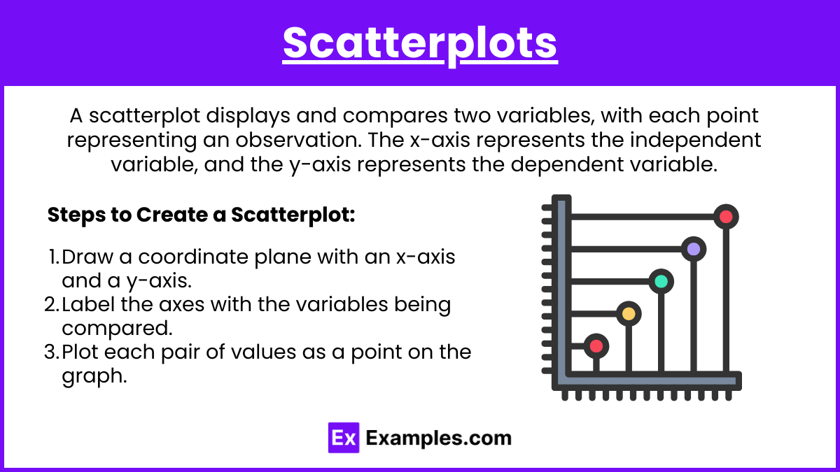
A scatterplot is a type of graph used to display and compare two variables. Each point on the scatterplot represents an observation from the data set. The x-axis typically represents the independent variable, while the y-axis represents the dependent variable.

Steps to Create a Scatterplot:

Draw a coordinate plane with an x-axis and a y-axis.
Label the axes with the variables being compared.
Plot each pair of values as a point on the graph.

Identifying Relationships in Scatterplots

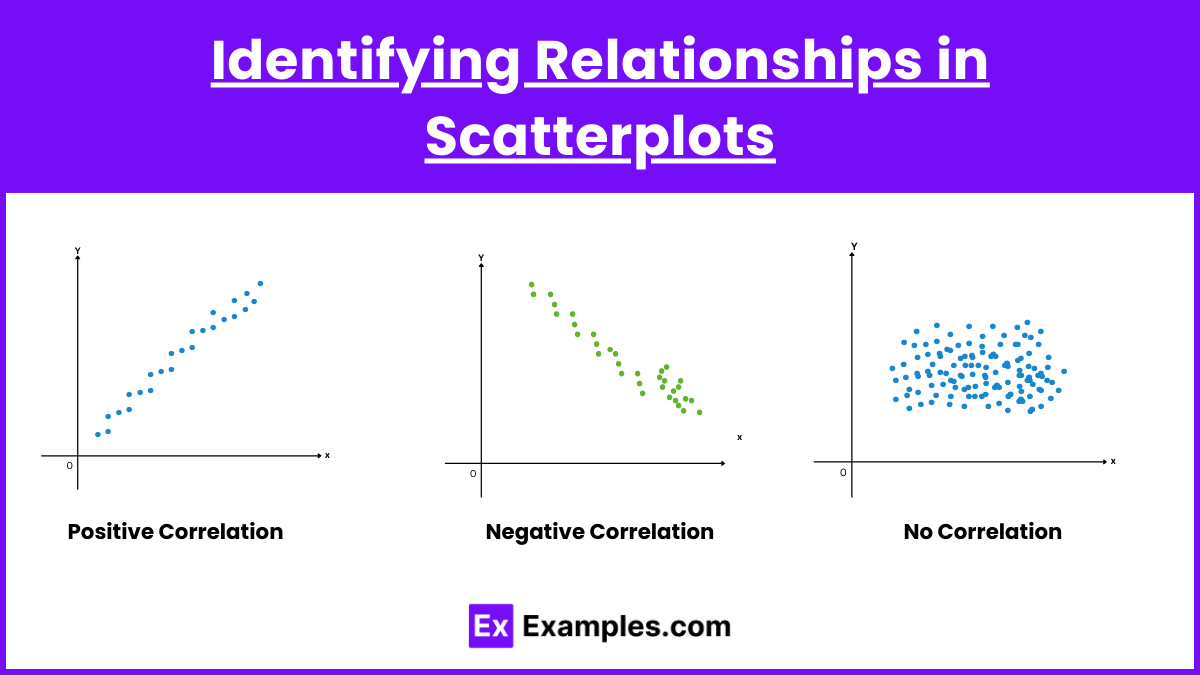
Scatterplots help identify the type of relationship between two variables. The relationship can be:

Positive Correlation: As the x-variable increases, the y-variable also increases.
Negative Correlation: As the x-variable increases, the y-variable decreases.
No Correlation: There is no apparent relationship between the x and y variables.

Models for Two-Variable Data

Once a relationship is identified, a mathematical model can be used to describe it. Common models include:

Linear Models

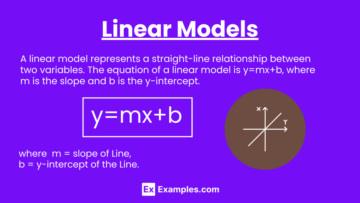
A linear model represents a straight-line relationship between two variables. The equation of a linear model is y=mx+b, where m is the slope and b is the y-intercept.

Steps to Create a Linear Model:

Calculate the slope \( m \) using the formula \( m = \frac{\sum{(x_i – \bar{x})(y_i – \bar{y})}}{\sum{(x_i – \bar{x})^2}} \)
Calculate the y-intercept \( b \) using \( b = \bar{y} – m\bar{x} \), where \( \bar{x} \) and \( \bar{y} \) are the means of the x and y values, respectively.
Write the equation y=mx+b.

Quadratic Models

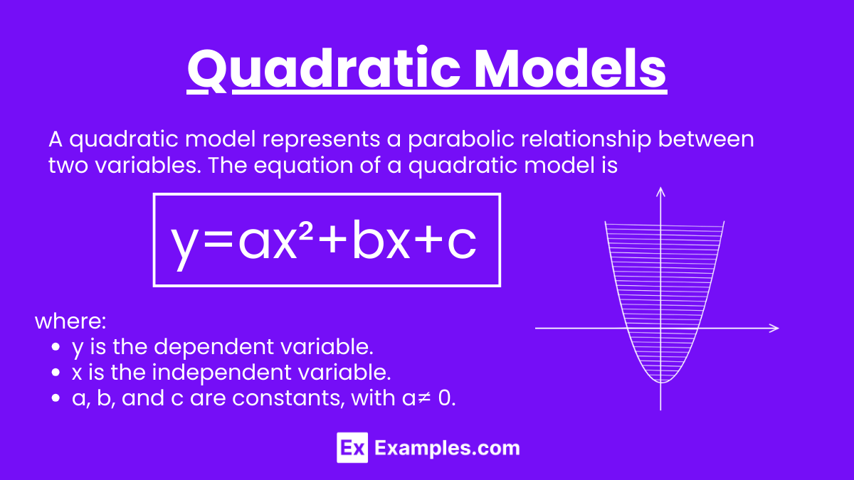
A quadratic model represents a parabolic relationship between two variables. The equation of a quadratic model is y=ax²+bx+c.

Steps to Create a Quadratic Model:

Use a system of equations to solve for the coefficients a, b, and c.
Substitute these values into the equation y=ax²+bx+c.

Exponential Models

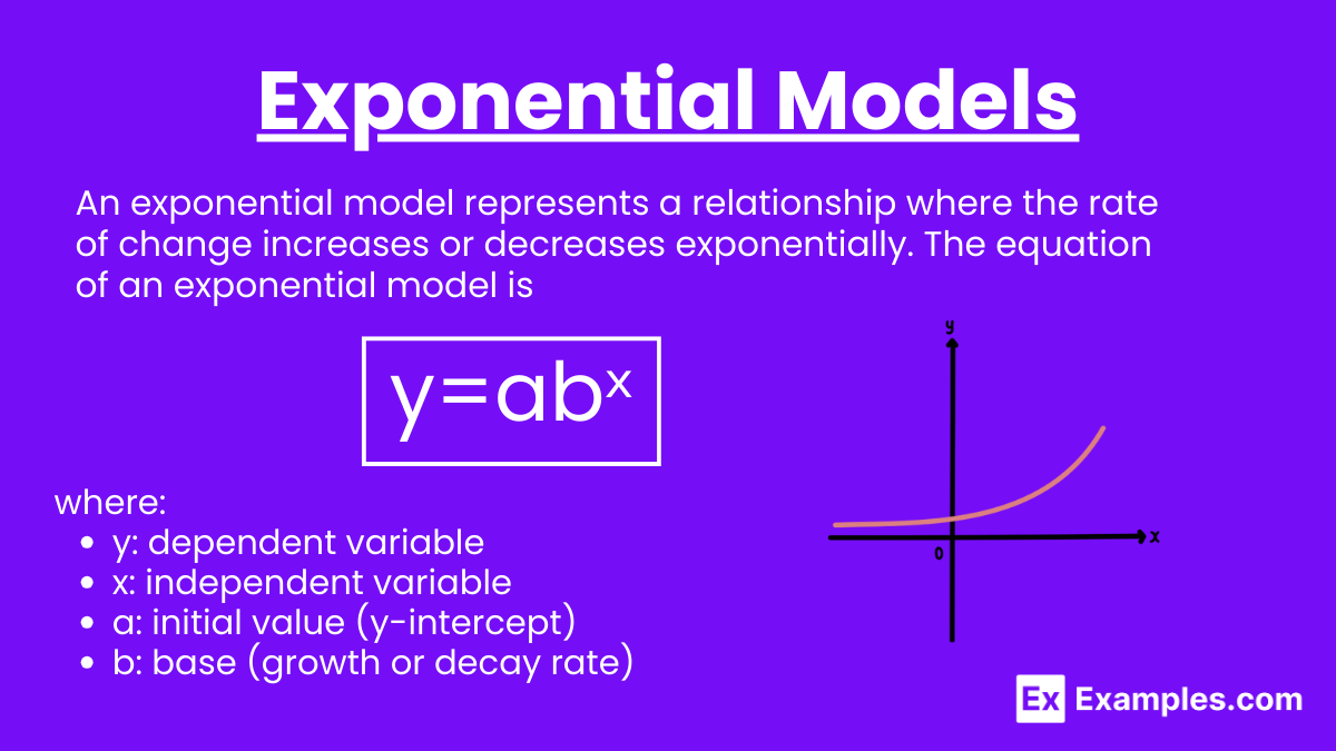
An exponential model represents a relationship where the rate of change increases or decreases exponentially. The equation of an exponential model is y=abˣ.

Steps to Create an Exponential Model:

Transform the data by taking the natural logarithm of the y-values.
Fit a linear model to the transformed data.
Convert the linear model back to the exponential form.

Interpreting Models and Making Predictions

Once a model is created, it can be used to make predictions. However, it is essential to understand the limitations and ensure the model fits the data well.

Residuals and Goodness of Fit:

Residuals: The differences between observed values and predicted values. Smaller residuals indicate a better fit.
Coefficient of Determination (R^2): A measure of how well the model explains the variability in the data. An R² value closer to 1 indicates a better fit.

Examples of Two-Variable Data: Models and Scatterplots

Example 1: Creating a Scatterplot

Given the data set:
(2,4),(3,9),(4,16),(5,25)
Create a scatterplot.

Draw the coordinate plane.
Label the x-axis as “X” and the y-axis as “Y”.
Plot the points on the graph.

Example 2: Linear Model

Given the data set: (1,2),(2,3),(3,5),(4,7)
Create a linear model.

Calculate the slope \( m \):
\( m = \frac{(1-2.5)(2-4.25) + (2-2.5)(3-4.25) + (3-2.5)(5-4.25) + (4-2.5)(7-4.25)}{(1-2.5)^2 + (2-2.5)^2 + (3-2.5)^2 + (4-2.5)^2} = \frac{9.5}{5} = 1.9 \)
Calculate the y-intercept b:
b=4.25−1.9⋅2.5=−0.5
The linear model is:
y=1.9x−0.5

Example 3: Quadratic Model

Given the data set: (1,2),(2,4),(3,10),(4,18)
Create a quadratic model.

Use the points to set up the system of equations: \( \begin{cases} a(1)^2 + b(1) + c = 2 \\ a(2)^2 + b(2) + c = 4 \\ a(3)^2 + b(3) + c = 10 \\ a(4)^2 + b(4) + c = 18 \end{cases} \).
Solve for a, b, and c:
a=1,b=0,c=1
The quadratic model is:
y=x²+1

Example 4: Exponential Model

Given the data set: (1,2),(2,4),(3,8),(4,16)
Create an exponential model.

Transform the data:
ln(2)=0.693,ln(4)=1.386,ln(8)=2.079,ln(16)=2.772
Fit a linear model to the transformed data:
y=0.693x
Convert back to the exponential form:
y=2ˣ

Example 5: Residuals and Goodness of Fit

Given the linear model y=2x+1 and the data set:
(1,3),(2,5),(3,7),(4,9)
Calculate the residuals and R2.

Calculate the predicted values:
(1,3),(2,5),(3,7),(4,9)
Calculate the residuals:
(3−3),(5−5),(7−7),(9−9)=0
Since all residuals are zero, R²=1, indicating a perfect fit.

Practice Questions

Question 1

Given the data set:
(1,3),(2,5),(3,7),(4,9)
Which of the following best represents the linear model for the data?

A) y=2x+1

B) y=3x+1

C) y=2x+2

D) y=3x+2

Answer: A

Explanation: To find the linear model, we use the slope formula \( m = \frac{(5-3)}{(2-1)} = 2 \). Using one of the points, such as (1,3), we substitute into \( y = mx + b \): \( 3 = 2(1) + b \), solving for \( b = 1 \). Thus, the linear model is \( y = 2x + 1 \).

Question 2

A scatterplot shows a positive correlation between two variables. Which of the following models is most likely appropriate?

A) Linear model y=mx+b

B) Quadratic model y=ax²+bx+c

C) Exponential model y=abˣ

D) Logarithmic model \( y = \log_b(x) \).

Answer: A

Explanation: A positive correlation in a scatterplot indicates that as one variable increases, the other also increases. A linear model y=mx+b is most appropriate for describing this linear relationship.

Question 3

Given the exponential model y=3⋅2ˣ, what is the value of y when x=4?

A) 12

B) 24

C) 48

D) 96

Answer: C

Explanation: Substitute x=4 into the exponential model: y=3⋅2⁴=3⋅16=48.
Therefore, the value of y when x=4 is 48.

Digital Sat