What is the root mean square (RMS) of the numbers 2, 3, and 4?
3.00
3.16
3.24
3.36
of 10

The Root Mean Square (RMS) is a statistical measure of the magnitude of a varying quantity, commonly used in fields such as physics, engineering, and statistics. It is calculated by taking the square and square root of the mean of the squares of a set of numbers, which can be integers, rational, or irrational numbers. This method aligns closely with algebraic principles, especially when involving square and square roots. RMS can also be integrated into the least squares method to minimize the sum of the squares of the errors. The concept is essential in data analysis, ensuring accurate and meaningful interpretations of complex datasets.
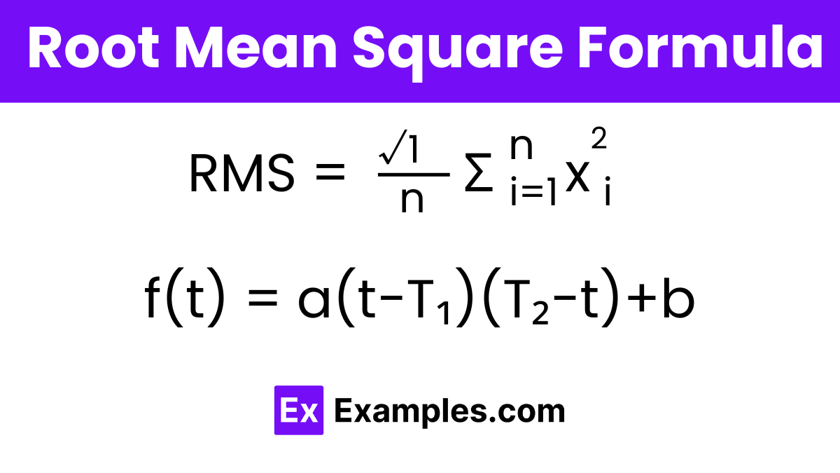
The Root Mean Square (RMS) is a mathematical measure used to calculate the average magnitude of a set of numbers, particularly useful in fields where we need to consider both the magnitude and duration of a varying quantity. Here’s the formula used to compute the RMS:
Calculate the RMS value of the following set of numbers: 2, 3, 6, 8, 11.
Square Each Number:
Sum the Squares:
Total = 4+9+36+64+121=234
Calculate the Mean of the Squares:
Since there are 5 numbers, the mean is 234/5 = 46.8
Take the Square Root of the Mean:
RMS = √46.8 = 6.84
The Root Mean Square of the numbers 2, 3, 6, 8, and 11 is approximately 6.84.
This example clearly demonstrates the process of calculating RMS from squaring each value, summing those squares, dividing by the number of data points to find the mean of the squares, and finally taking the square root of that mean. RMS calculations are particularly useful for understanding the effective magnitude of various datasets, especially in fields like electrical engineering, acoustics, and physics.
To provide a formula for a continuous function 𝑓(𝑡) defined over an interval 𝑇₁≤𝑡≤𝑇₂, we need more specific details about the function’s behavior or the rules it follows within that interval. However, without specific details, we can consider general forms and representations that could apply to such a function.
a and 𝑏b are constants that can be adjusted based on additional conditions or constraints you might have (like values at endpoints or specific behavior at points within the interval).This form ensures f(t) is continuous and zero at T₁ and 𝑇₂ if b = 0. Adjust 𝑏b if a different value is needed at the boundaries. Polynomial Representation A polynomial function is always a good choice for a continuous function over a closed interval due to its inherent smoothness and ease of integration differentiation: f(t) = c₀ + c₁t + c₂t² + ⋯ + cₙtⁿ and c₀c₁…cₙ are coefficients that determine the shape and behavior of the polynomial. Trigonometric Representation If the function needs to exhibit periodic behavior within T₁ and 𝑇₂, a trigonometric form might be suitable: f(t)=Asin(ωt+ϕ)+B𝐴, 𝜔, and ϕ control the amplitude, frequency, and phase of the wave, respectively.𝐵 adjusts the baseline of the sinusoidal wave. Exponential or Logarithmic Forms For growth or decay types of continuous functions, consider exponential or logarithmic forms: 𝑓(𝑡) = 𝐶exp(𝐷(𝑡−𝑇1))f(t) = 𝐸log(𝑡−𝑇1+𝐹)C, D, E, and F are constants that need to be determined based on specific behavior or boundary conditions.
Suppose you need a continuous function 𝑓(𝑡) that is defined over the interval 0≤𝑡≤5 and has specific values at the endpoints. Let’s say 𝑓(0) = 2 and 𝑓(5) = 10. We’ll use a quadratic polynomial because it’s simple yet can easily meet these conditions.
A general quadratic polynomial can be expressed as: 𝑓(𝑡) = 𝑎𝑡²+𝑏𝑡+𝑐
Boundary Conditions:
Setting Up Equations:
From 𝑓(5) = 10, substituting 𝑐 = 2:
Choosing a Value: For simplicity, let’s assume 𝑎=0.4. Then,
With 𝑎 = 0.4, 𝑏 = −0.4, and 𝑐 = 2, our function is:
𝑓(𝑡) = 0.4𝑡²−0.4𝑡+2
Let’s calculate 𝑓(𝑡) at a few points within the interval:
At 𝑡=0:
𝑓(0) = 0.4⋅0²−0.4⋅0+2 = 2
At 𝑡=5:
𝑓(5) = 0.4⋅5²−0.4⋅5+2=10
At 𝑡=2.5 (midpoint):
𝑓(2.5) = 0.4⋅2.5²−0.4⋅2.5+2 = 2.5−1+2 = 3.5
This example illustrates how to define a simple polynomial function with specific boundary conditions. By adjusting the coefficients 𝑎, 𝑏, and 𝑐, you can tailor the function to meet various other conditions and behaviors over any specified interval.
To calculate the Root Mean Square (RMS) of a set of numbers, follow these steps:
Yes, RMS can be applied to any set of real numbers. It is particularly useful for data sets where values change direction around a central point, like sound waves or financial market prices.
The main difference between RMS and the arithmetic mean is that RMS gives a higher weight to larger numbers due to the squaring process. This makes RMS more sensitive to outliers and extreme values than the arithmetic mean, which could be more representative of data sets with large fluctuations.

What is the root mean square (RMS) of the numbers 2, 3, and 4?
3.00
3.16
3.24
3.36
What is the RMS value of the numbers 1, 2, and 3?
1.87
2.00
2.24
2.45
Calculate the RMS of the numbers 4, 5, and 6
4.92
5.00
5.45
5.70
What is the RMS value of the numbers 7 and 8?
7.81
7.28
7.27
7.29
What is the RMS of 5, 7, and 9?
6.60
7.00
8.50
7.80
Calculate the RMS of 3, 6, and 9.
5.76
6.71
6.00
7.00
What is the RMS value for the numbers 2, 4, and 6?
3.87
4.00
4.47
4.82
What is the RMS of the numbers 1, 3, and 5?
3.32
3.16
2.83
2.55
Calculate the RMS value for 8 and 10.
8.94
9.00
9.22
9.49
What is the RMS value for the numbers 4, 8, and 12?
6.00
6.93
7.48
7.93