What is the kinematic equation used to calculate the final velocity of an object when the initial velocity, acceleration, and time are known?
v=u+atv=u+at
s=ut+12at2s=ut+12at2
v2=u2+2asv2=u2+2as
s=vt−12at2s=vt−12at2
of 10

Kinematic equations are fundamental tools in physics used to describe the motion of objects. These equations relate various aspects of motion, such as displacement, velocity, acceleration, and time, without considering the forces causing the motion. By understanding and applying kinematic equations, we can predict and analyze the behavior of objects in motion, whether they are moving in a straight line or along a curved path. These equations form the basis for solving problems in mechanics, allowing us to explore everything from the trajectory of a projectile to the motion of a car on a highway.
Kinematic equations describe the motion of objects under constant acceleration. They relate displacement, velocity, acceleration, and time. An example is ( v = u + at ), where ( v ) is final velocity, ( u ) is initial velocity, ( a ) is acceleration, and ( t ) is time.
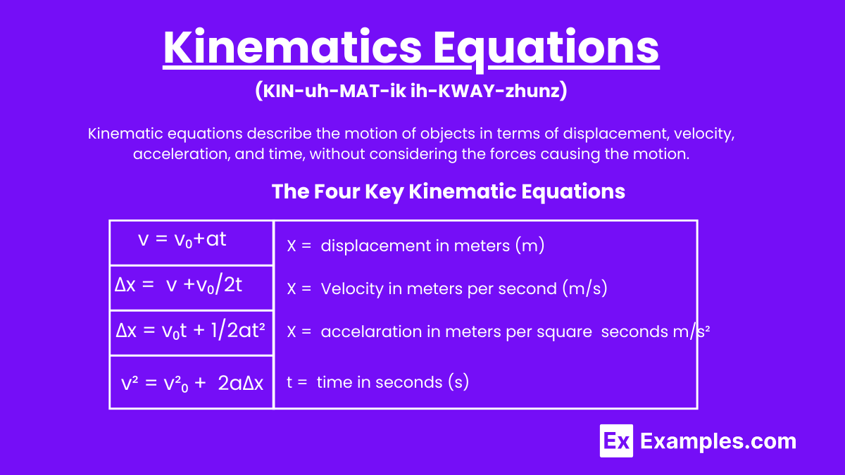
There are four basic kinematics equations:

This physics equation can be interpreted as: “The final velocity equals the initial velocity plus the product of acceleration and time.” Essentially, it means that if an object experiences constant acceleration over a given period, you can determine its final velocity. This equation is particularly useful when analyzing situations involving changing velocities under constant acceleration.
This equation is expressed as: “Displacement equals the sum of the final velocity and the initial velocity, divided by two, multiplied by time.” It is used when acceleration is not given, but you need to connect changing velocity with displacement.
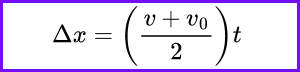
This equation may appear more complex due to its length, but it is read as: “Displacement equals initial velocity times time plus one-half of acceleration times time squared.” Essentially, it means that displacement can be determined using initial velocity and constant acceleration, without needing the final velocity. This equation is useful when the final velocity is the only unknown value.
There is another common form of this kinematic equation:
[ x = x₀ + v₀t + 1/2at²]
Although it may seem more daunting, it is essentially the same equation. The difference is that Δx has been split into (x – x₀), and then solved for (x). This version can be particularly useful when you need to find a specific final or initial position rather than just the overall displacement.
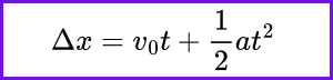
Our final kinematic equation is expressed as: “Final velocity squared equals initial velocity squared plus two times acceleration times displacement.” Notably, this is the only kinematic equation that does not include time. Many beginning physics students are often perplexed when they encounter problems that do not provide a time value. While an equation sheet filled with symbols and numbers can be intimidating, remembering this particular equation can be extremely helpful, as it frequently comes into play in various physics scenarios.
It’s important to note that all these equations apply to situations with constant acceleration. While this may seem like a limitation, high school physics typically focuses on constant acceleration, so you don’t need to worry about changing acceleration at this stage. If you advance to more complex courses, you will be introduced to additional physics equations that account for varying acceleration as needed.
1.) To begin deriving the first kinematic equation, we should first consider the definition of acceleration.𝑎=Δ𝑣/Δ𝑡
2.) We know Δ𝑣 = 𝑣−𝑣₀ , and when we plug that in, we get 𝑎=𝑣−𝑣₀/Δ𝑡
3.) If we solve for 𝑣, the equation becomes 𝑣 = 𝑣₀ + 𝑎Δ𝑡
4.) We can denote the time interval as t to generate the first kinematic equation.

Here’s a refined explanation of the calculations leading to the second kinematic equation:
1. The height of the blue rectangle is ( v₀) and the width is ( t ), so the area is equal to ( v₀ t ).
2. The base of the red triangle is ( t ) and the height is ( v – v₀ ), so the area of the red triangle is 1/2(v – v₀)t
3. When we sum the areas of the red triangle and the blue rectangle, we get:
[ v₀t + 1/2(v – v₀) t]
4. Distributing the factor of  in the red triangle area, we have:
[ v₀t + 1/2at²]
5. We can simplify the equation by combining the initial velocity terms:
s = v₀t + 1/2at²
This leads us to the second kinematic equation, which expresses the displacement ( s ) in terms of initial velocity (v₀), acceleration ( a ), and time ( t ).

We can derive the third kinematic equation by plugging the first kinematic equation into the second kinematic equation. Here’s how:
1. Start with the second kinematic equation:
[ s = v₀t +1/2at²]
2. Substitute the first kinematic equation \( v = v₀ + at ) for (v )
[ s = v₀ t + 1/2 (v – v₀) t ]
3. Once substituted, the equation becomes:
[ s = v₀t + 1/2 (v₀ + at – v₀)t ]
4. Expand the equation:
[ s = v₀t + 1/2at² ]
5. Combine terms to simplify the equation:
[ s = v₀t + 1/2at² ]
6. Finally, multiply both sides by 2 to eliminate the fraction:
[ 2s = 2v₀t + at² ]
Rearrange to get the third kinematic equation:
[ v² = v₀² + 2as ]
This is the third kinematic equation, which relates the final velocity squared to the initial velocity squared, acceleration, and displacement.

The fourth kinematic equation can be derived using the first and second kinematic equations. Here’s how:
Start with the second kinematic equation: [ s = v₀t + 1/2at² ]
Use the first kinematic equation ( v = v₀ + at ) to solve for time ( t ): [ t = v – v₀/a ]
Substitute this expression for ( t ) into the second kinematic equation: [ s = v₀ (v-v₀/a) + 1/2a(v-v₀/a)²
Multiply the fractions to simplify the equation: [ s = v₀(v-v₀)/a + 1/2a((v-v₀/a²)²)
Simplify further to solve for ( s ): [ s = v₀(v-v₀) + 1/2 (v-v₀)²/a
s = v₀(v-v₀) + 1/2(v²-2v₀v+v₀²/a
s =v₀v-v² + 1/2v²-v₀v+1/2v₀²/a
s = 1/2v² – v₀²/a
s = 1/2v² – v₀²/a
2as = v²−v₀²
Finally, solve for ( v² )
[ v² = v₀² + 2as ]
This is the fourth kinematic equation, relating the final velocity squared to the initial velocity squared, acceleration, and displacement.
In projectile motion, the kinematic equations describe the horizontal and vertical components of an object’s motion separately. One of the key equations for projectile motion is the equation for the vertical displacement:
[ y = v₀ᵧt – 1/2gt² ]
This equation describes the vertical position (y) of a projectile at any time (t) during its flight. The term (v₀ᵧ) represents the initial vertical velocity, which is the component of the initial velocity in the vertical direction. The gravitational acceleration (g) is a constant (approximately (9.8m/s²) on Earth) that acts downward, hence the negative sign. The term (1/2gt²) accounts for the displacement due to gravity over time.
This equation helps determine the height of a projectile at any point in time, considering both its initial upward velocity and the downward pull of gravity. It is essential for analyzing the vertical aspect of projectile motion, such as determining the maximum height reached or the time it takes for the projectile to hit the ground.
One of the fundamental kinematic equations for motion under constant acceleration is:
[ v = v₀ + at ]
This equation connects the final velocity (v) of an object to its initial velocity (v₀ ), the constant acceleration (a), and the time (t) over which the acceleration occurs. The initial velocity ((v_0)) is the speed at which the object starts, and the acceleration (a) is the rate of change of velocity. By multiplying the acceleration by the time, we determine the change in velocity. Adding this change to the initial velocity gives the final velocity.
This equation is widely used in physics to analyze the motion of objects under constant acceleration. It helps in calculating the final speed of vehicles accelerating on a straight path, determining the velocity of a falling object at any given time, or finding the speed of a rocket shortly after launch. By providing a direct relationship between velocity, acceleration, and time, this equation is essential for solving problems involving linear motion with uniform acceleration.
Identify Known and Unknown Variables:
Determine which variables are given (initial velocity (v₀), final velocity (v), acceleration (a), time (t), displacement (s)) and which one you need to find.
Select the Appropriate Equation:
Choose the kinematic equation that includes the known variables and the unknown variable you need to solve for. Common equations are:
( v = v₀ + at )
( s = v₀t +1/2 at² )
( v² = v₀² + 2as )
( s =v+v₀/2t )
Rearrange the Equation:
If necessary, rearrange the equation to solve for the unknown variable. For example, to find (t) from ( v = v₀ + at ), rearrange to ( t = v-v₀/a ).
Substitute Known Values:
Plug the known values into the equation.
Solve the Equation:
Perform the arithmetic operations to solve for the unknown variable.
Check Units and Reasonableness:
Ensure your answer has the correct units and check if it makes sense in the context of the problem.
Final Velocity:
[ v = v₀ + at ]
This equation calculates the final velocity ((v)) given the initial velocity ((v_0)), acceleration ((a)), and time ((t)).
Displacement (using initial velocity and time):
[ s = v₀t + 1/2 at² ]
This equation determines the displacement ((s)) using the initial velocity, acceleration, and time.
Displacement (using average velocity):
[ s =v₀t+1/2at² ]
This calculates displacement using the average of the initial and final velocities and time.
Final Velocity (using displacement):
[ v² = v₀² + 2as ]
This equation relates the final velocity squared to the initial velocity squared, acceleration, and displacement.
These equations are used to solve various motion problems by identifying known variables and selecting the appropriate formula to find unknown quantities. They are foundational in classical mechanics for predicting and understanding object motion.
Displacement (s or Δx):
The change in position of an object. It is a vector quantity, meaning it has both magnitude and direction.
Initial Velocity (v₀) or (u):
The velocity of an object at the start of the time interval being considered. It is a vector quantity.
Final Velocity (v):
The velocity of an object at the end of the time interval being considered. It is also a vector quantity.
Acceleration (a):
The rate at which an object’s velocity changes with time. It is a vector quantity and can be positive (speeding up) or negative (slowing down).
Time (t):
The duration over which the motion occurs. It is a scalar quantity, meaning it only has magnitude and no direction.
These quantities are used in the kinematic equations to analyze and predict the motion of objects under constant acceleration.
The image depicts two cars on a road in a clean, technical illustration. On the left, a car labeled “initial velocity (at rest)” indicates the starting point with an arrow showing an acceleration of 4.5 m/s². On the right, a car labeled “velocity after 10 sec?” represents the final situation. Below each car, the terms “initial situation” and “final situation” are indicated. The design includes labeled axes and lines suggesting motion and acceleration, emphasizing the calculation of the car’s velocity after a given period, making it a clear representation of kinematic principles.
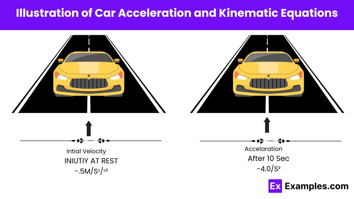
This illustration demonstrates a basic kinematic scenario where a car initially at rest accelerates at 4.5 m/s². It shows how to calculate the car’s velocity after 10 seconds, emphasizing the relationship between initial velocity, acceleration, and time in determining the final velocity.
These rotational kinematics equations are essentially corollaries of the linear kinematics equations, with the variables changed accordingly:
| Rotational Motion (α = constant) | Linear Motion (a = constant) |
|---|---|
| 𝜔 = 𝜔₀ + 𝛼𝑡 | 𝑣 = 𝑣₀ + 𝑎𝑡 |
| Θ = 1/2( 𝜔 + 𝜔₀ )𝑡 | 𝑥 = 1/2(𝑣₀ + 𝑣)𝑡 |
| Θ = 𝜔₀𝑡+1/2𝛼𝑡² | 𝑥 = 𝑣₀𝑡 +12𝑎𝑡² |
| 𝜔2 = 𝜔²₀ + 2𝛼Θ | 𝑣2 = 𝑣²₀+ 2𝑎𝑥 |
Initial velocity is the starting speed of an object. It affects the object’s future velocity, displacement, and the outcome of the motion when combined with acceleration and time.
Time is the duration over which the motion occurs. It links how long an object has been moving with changes in velocity and displacement.
Displacement is the straight-line distance between the starting and ending points with direction, while distance is the total path length traveled regardless of direction.
Identify the known and unknown variables.
Choose the appropriate kinematic equation.
Substitute the known values into the equation.
Solve for the unknown variable
The first kinematic equation is 𝑣=𝑢+𝑎𝑡, where 𝑣v is the final velocity, 𝑢u is the initial velocity, 𝑎a is the acceleration, and 𝑡t is the time.
Kinematic equations can be used when the acceleration is constant.
Yes, kinematic equations can be adapted to rotational motion by replacing linear variables with their rotational counterparts (e.g., angular displacement, angular velocity, angular acceleration).
Displacement can be calculated using any of the kinematic equations, depending on the known variables (e.g., initial and final velocities, acceleration, and time).
Yes, kinematic equations can be applied to free-fall problems by considering the acceleration due to gravity.
The units of angular displacement are radians (rad) or degrees (°), but radians are more commonly used in physics.

Kinematic equations are fundamental tools in physics used to describe the motion of objects. These equations relate various aspects of motion, such as displacement, velocity, acceleration, and time, without considering the forces causing the motion. By understanding and applying kinematic equations, we can predict and analyze the behavior of objects in motion, whether they are moving in a straight line or along a curved path. These equations form the basis for solving problems in mechanics, allowing us to explore everything from the trajectory of a projectile to the motion of a car on a highway.
Kinematic equations describe the motion of objects under constant acceleration. They relate displacement, velocity, acceleration, and time. An example is ( v = u + at ), where ( v ) is final velocity, ( u ) is initial velocity, ( a ) is acceleration, and ( t ) is time.
There are four basic kinematics equations:
This physics equation can be interpreted as: “The final velocity equals the initial velocity plus the product of acceleration and time.” Essentially, it means that if an object experiences constant acceleration over a given period, you can determine its final velocity. This equation is particularly useful when analyzing situations involving changing velocities under constant acceleration.
This equation is expressed as: “Displacement equals the sum of the final velocity and the initial velocity, divided by two, multiplied by time.” It is used when acceleration is not given, but you need to connect changing velocity with displacement.
This equation may appear more complex due to its length, but it is read as: “Displacement equals initial velocity times time plus one-half of acceleration times time squared.” Essentially, it means that displacement can be determined using initial velocity and constant acceleration, without needing the final velocity. This equation is useful when the final velocity is the only unknown value.
There is another common form of this kinematic equation:
[ x = x₀ + v₀t + 1/2at²]
Although it may seem more daunting, it is essentially the same equation. The difference is that Δx has been split into (x – x₀), and then solved for (x). This version can be particularly useful when you need to find a specific final or initial position rather than just the overall displacement.
Our final kinematic equation is expressed as: “Final velocity squared equals initial velocity squared plus two times acceleration times displacement.” Notably, this is the only kinematic equation that does not include time. Many beginning physics students are often perplexed when they encounter problems that do not provide a time value. While an equation sheet filled with symbols and numbers can be intimidating, remembering this particular equation can be extremely helpful, as it frequently comes into play in various physics scenarios.
It’s important to note that all these equations apply to situations with constant acceleration. While this may seem like a limitation, high school physics typically focuses on constant acceleration, so you don’t need to worry about changing acceleration at this stage. If you advance to more complex courses, you will be introduced to additional physics equations that account for varying acceleration as needed.
1.) To begin deriving the first kinematic equation, we should first consider the definition of acceleration.𝑎=Δ𝑣/Δ𝑡
2.) We know Δ𝑣 = 𝑣−𝑣₀ , and when we plug that in, we get 𝑎=𝑣−𝑣₀/Δ𝑡
3.) If we solve for 𝑣, the equation becomes 𝑣 = 𝑣₀ + 𝑎Δ𝑡
4.) We can denote the time interval as t to generate the first kinematic equation.
Here’s a refined explanation of the calculations leading to the second kinematic equation:
1. The height of the blue rectangle is ( v₀) and the width is ( t ), so the area is equal to ( v₀ t ).
2. The base of the red triangle is ( t ) and the height is ( v – v₀ ), so the area of the red triangle is 1/2(v – v₀)t
3. When we sum the areas of the red triangle and the blue rectangle, we get:
[ v₀t + 1/2(v – v₀) t]
4. Distributing the factor of in the red triangle area, we have:
[ v₀t + 1/2at²]
5. We can simplify the equation by combining the initial velocity terms:
s = v₀t + 1/2at²
This leads us to the second kinematic equation, which expresses the displacement ( s ) in terms of initial velocity (v₀), acceleration ( a ), and time ( t ).
We can derive the third kinematic equation by plugging the first kinematic equation into the second kinematic equation. Here’s how:
1. Start with the second kinematic equation:
[ s = v₀t +1/2at²]
2. Substitute the first kinematic equation \( v = v₀ + at ) for (v )
[ s = v₀ t + 1/2 (v – v₀) t ]
3. Once substituted, the equation becomes:
[ s = v₀t + 1/2 (v₀ + at – v₀)t ]
4. Expand the equation:
[ s = v₀t + 1/2at² ]
5. Combine terms to simplify the equation:
[ s = v₀t + 1/2at² ]
6. Finally, multiply both sides by 2 to eliminate the fraction:
[ 2s = 2v₀t + at² ]
Rearrange to get the third kinematic equation:
[ v² = v₀² + 2as ]
This is the third kinematic equation, which relates the final velocity squared to the initial velocity squared, acceleration, and displacement.
The fourth kinematic equation can be derived using the first and second kinematic equations. Here’s how:
Start with the second kinematic equation: [ s = v₀t + 1/2at² ]
Use the first kinematic equation ( v = v₀ + at ) to solve for time ( t ): [ t = v – v₀/a ]
Substitute this expression for ( t ) into the second kinematic equation: [ s = v₀ (v-v₀/a) + 1/2a(v-v₀/a)²
Multiply the fractions to simplify the equation: [ s = v₀(v-v₀)/a + 1/2a((v-v₀/a²)²)
Simplify further to solve for ( s ): [ s = v₀(v-v₀) + 1/2 (v-v₀)²/a
s = v₀(v-v₀) + 1/2(v²-2v₀v+v₀²/a
s =v₀v-v² + 1/2v²-v₀v+1/2v₀²/a
s = 1/2v² – v₀²/a
s = 1/2v² – v₀²/a
2as = v²−v₀²
Finally, solve for ( v² )
[ v² = v₀² + 2as ]
This is the fourth kinematic equation, relating the final velocity squared to the initial velocity squared, acceleration, and displacement.
In projectile motion, the kinematic equations describe the horizontal and vertical components of an object’s motion separately. One of the key equations for projectile motion is the equation for the vertical displacement:
[ y = v₀ᵧt – 1/2gt² ]
This equation describes the vertical position (y) of a projectile at any time (t) during its flight. The term (v₀ᵧ) represents the initial vertical velocity, which is the component of the initial velocity in the vertical direction. The gravitational acceleration (g) is a constant (approximately (9.8m/s²) on Earth) that acts downward, hence the negative sign. The term (1/2gt²) accounts for the displacement due to gravity over time.
This equation helps determine the height of a projectile at any point in time, considering both its initial upward velocity and the downward pull of gravity. It is essential for analyzing the vertical aspect of projectile motion, such as determining the maximum height reached or the time it takes for the projectile to hit the ground.
One of the fundamental kinematic equations for motion under constant acceleration is:
[ v = v₀ + at ]
This equation connects the final velocity (v) of an object to its initial velocity (v₀ ), the constant acceleration (a), and the time (t) over which the acceleration occurs. The initial velocity ((v_0)) is the speed at which the object starts, and the acceleration (a) is the rate of change of velocity. By multiplying the acceleration by the time, we determine the change in velocity. Adding this change to the initial velocity gives the final velocity.
This equation is widely used in physics to analyze the motion of objects under constant acceleration. It helps in calculating the final speed of vehicles accelerating on a straight path, determining the velocity of a falling object at any given time, or finding the speed of a rocket shortly after launch. By providing a direct relationship between velocity, acceleration, and time, this equation is essential for solving problems involving linear motion with uniform acceleration.
Identify Known and Unknown Variables:
Determine which variables are given (initial velocity (v₀), final velocity (v), acceleration (a), time (t), displacement (s)) and which one you need to find.
Select the Appropriate Equation:
Choose the kinematic equation that includes the known variables and the unknown variable you need to solve for. Common equations are:
( v = v₀ + at )
( s = v₀t +1/2 at² )
( v² = v₀² + 2as )
( s =v+v₀/2t )
Rearrange the Equation:
If necessary, rearrange the equation to solve for the unknown variable. For example, to find (t) from ( v = v₀ + at ), rearrange to ( t = v-v₀/a ).
Substitute Known Values:
Plug the known values into the equation.
Solve the Equation:
Perform the arithmetic operations to solve for the unknown variable.
Check Units and Reasonableness:
Ensure your answer has the correct units and check if it makes sense in the context of the problem.
Final Velocity:
[ v = v₀ + at ]
This equation calculates the final velocity ((v)) given the initial velocity ((v_0)), acceleration ((a)), and time ((t)).
Displacement (using initial velocity and time):
[ s = v₀t + 1/2 at² ]
This equation determines the displacement ((s)) using the initial velocity, acceleration, and time.
Displacement (using average velocity):
[ s =v₀t+1/2at² ]
This calculates displacement using the average of the initial and final velocities and time.
Final Velocity (using displacement):
[ v² = v₀² + 2as ]
This equation relates the final velocity squared to the initial velocity squared, acceleration, and displacement.
These equations are used to solve various motion problems by identifying known variables and selecting the appropriate formula to find unknown quantities. They are foundational in classical mechanics for predicting and understanding object motion.
Displacement (s or Δx):
The change in position of an object. It is a vector quantity, meaning it has both magnitude and direction.
Initial Velocity (v₀) or (u):
The velocity of an object at the start of the time interval being considered. It is a vector quantity.
Final Velocity (v):
The velocity of an object at the end of the time interval being considered. It is also a vector quantity.
Acceleration (a):
The rate at which an object’s velocity changes with time. It is a vector quantity and can be positive (speeding up) or negative (slowing down).
Time (t):
The duration over which the motion occurs. It is a scalar quantity, meaning it only has magnitude and no direction.
These quantities are used in the kinematic equations to analyze and predict the motion of objects under constant acceleration.
The image depicts two cars on a road in a clean, technical illustration. On the left, a car labeled “initial velocity (at rest)” indicates the starting point with an arrow showing an acceleration of 4.5 m/s². On the right, a car labeled “velocity after 10 sec?” represents the final situation. Below each car, the terms “initial situation” and “final situation” are indicated. The design includes labeled axes and lines suggesting motion and acceleration, emphasizing the calculation of the car’s velocity after a given period, making it a clear representation of kinematic principles.
This illustration demonstrates a basic kinematic scenario where a car initially at rest accelerates at 4.5 m/s². It shows how to calculate the car’s velocity after 10 seconds, emphasizing the relationship between initial velocity, acceleration, and time in determining the final velocity.
These rotational kinematics equations are essentially corollaries of the linear kinematics equations, with the variables changed accordingly:
Displacement is replaced by angular displacement.
Initial and final velocities are replaced by initial and final angular velocities.
Acceleration is replaced by angular acceleration.
Time remains the constant factor.
Rotational Motion (α = constant) | Linear Motion (a = constant) |
|---|---|
𝜔 = 𝜔₀ + 𝛼𝑡 | 𝑣 = 𝑣₀ + 𝑎𝑡 |
Θ = 1/2( 𝜔 + 𝜔₀ )𝑡 | 𝑥 = 1/2(𝑣₀ + 𝑣)𝑡 |
Θ = 𝜔₀𝑡+1/2𝛼𝑡² | 𝑥 = 𝑣₀𝑡 +12𝑎𝑡² |
𝜔2 = 𝜔²₀ + 2𝛼Θ | 𝑣2 = 𝑣²₀+ 2𝑎𝑥 |
Initial velocity is the starting speed of an object. It affects the object’s future velocity, displacement, and the outcome of the motion when combined with acceleration and time.
Time is the duration over which the motion occurs. It links how long an object has been moving with changes in velocity and displacement.
Displacement is the straight-line distance between the starting and ending points with direction, while distance is the total path length traveled regardless of direction.
Identify the known and unknown variables.
Choose the appropriate kinematic equation.
Substitute the known values into the equation.
Solve for the unknown variable
The first kinematic equation is 𝑣=𝑢+𝑎𝑡, where 𝑣v is the final velocity, 𝑢u is the initial velocity, 𝑎a is the acceleration, and 𝑡t is the time.
Kinematic equations can be used when the acceleration is constant.
Yes, kinematic equations can be adapted to rotational motion by replacing linear variables with their rotational counterparts (e.g., angular displacement, angular velocity, angular acceleration).
Displacement can be calculated using any of the kinematic equations, depending on the known variables (e.g., initial and final velocities, acceleration, and time).
Yes, kinematic equations can be applied to free-fall problems by considering the acceleration due to gravity.
The units of angular displacement are radians (rad) or degrees (°), but radians are more commonly used in physics.
What is the kinematic equation used to calculate the final velocity of an object when the initial velocity, acceleration, and time are known?
v=u+atv=u+at
s=ut+12at2s=ut+12at2
v2=u2+2asv2=u2+2as
s=vt−12at2s=vt−12at2
Which kinematic equation relates displacement, initial velocity, acceleration, and time?
v=u+atv=u+at
s=ut+12at2s=ut+12at2
v2=u2+2asv2=u2+2as
s=vt−12at2s=vt−12at2
Which kinematic equation can be used to find acceleration when initial velocity, final velocity, and displacement are given?
v=u+atv=u+at
s=ut+12at2s=ut+12at2
v2=u2+2asv2=u2+2as
s=vt−12at2s=vt−12at2
In the equation v2=u2+2asv2=u2+2as, what does ss represent?
Time
Displacement
Initial velocity
Final velocity
How is the average velocity vavgvavg calculated when acceleration is constant?
vavg=v+u2vavg=v+u2
vavg=v−uvavg=v−u
vavg=u2vavg=u2
vavg=stvavg=st
Which kinematic equation can be used to find the time of travel when initial velocity, final velocity, and acceleration are known?
v=u+atv=u+at
s=ut+12at2s=ut+12at2
v2=u2+2asv2=u2+2as
s=vt−12at2s=vt−12at2
If an object starts from rest and accelerates uniformly at 5 m/s², what is its velocity after 4 second
10 m/s
20 m/s
15 m/s
5 m/s
An object is thrown upwards with an initial velocity of 30 m/s. What is its displacement after 3 seconds, assuming acceleration due to gravity is −9.8m/s2−9.8m/s2?
75 m
45 m
90 m
120 m
If the displacement of an object is 100 meters, and its initial velocity is 10 m/s with an acceleration of 2 m/s², what is its final velocity after covering this distance?
30 m/s
40 m/s
25 m/s
20 m/s
How can the displacement be calculated if you know the average velocity and time?
s=vavg×ts=vavg×t
s=vavgts=vavgt
s=vavg+ts=vavg+t
s=vavg−ts=vavg−t